Graph durch Euler

This is the famous Ulam spiral, in which prime numbers are represented on filled squares on a square spiral:

The Ulam spiral


I like the way the spiral sits between chaos and calm. It’s not wholly random and it’s not wholly regular — it’s betwixt and between. You get a similar chaos-and-calm vibe from a graph for a function called Euler phi. And primes are at work there too. Here’s the graph from Wikipedia:

Graph of eulerphi(n) = φ(n) (see Euler’s totient function)


But what is the Euler phi function? For any integer n, eulerphi(n) gives you the count of numbers < n that are relatively prime to n. That is, the count of numbers < n that have no common factors with n other than one. You can see how eulerphi(n) works by considering whether you can simplify the fraction a/b, where a = 1..n-1 and b = n:

φ(6) = 2
1/6 (1)
2/6 → 1/3
3/6 → 1/2
4/6 → 2/3
5/6, ∴ φ(6) = 2


φ(7) = 6
1/7 (1)
2/7 (2)
3/7 (3)
4/7 (4)
5/7 (5)
6/7, ∴ φ(7) = 6


φ(12) = 4
1/12 (1)
2/12 → 1/6
3/12 → 1/4
4/12 → 1/3
5/12 (2)
6/12 → 1/2
7/12 (3)
8/12 → 2/3
9/12 → 3/4
10/12 → 5/6
11/12, ∴ φ(12) = 4


φ(13) = 12
1/13 (1)
2/13 (2)
3/13 (3)
4/13 (4)
5/13 (5)
6/13 (6)
7/13 (7)
8/13 (8)
9/13 (9)
10/13 (10)
11/13 (11)
12/13, ∴ φ(13) = 12


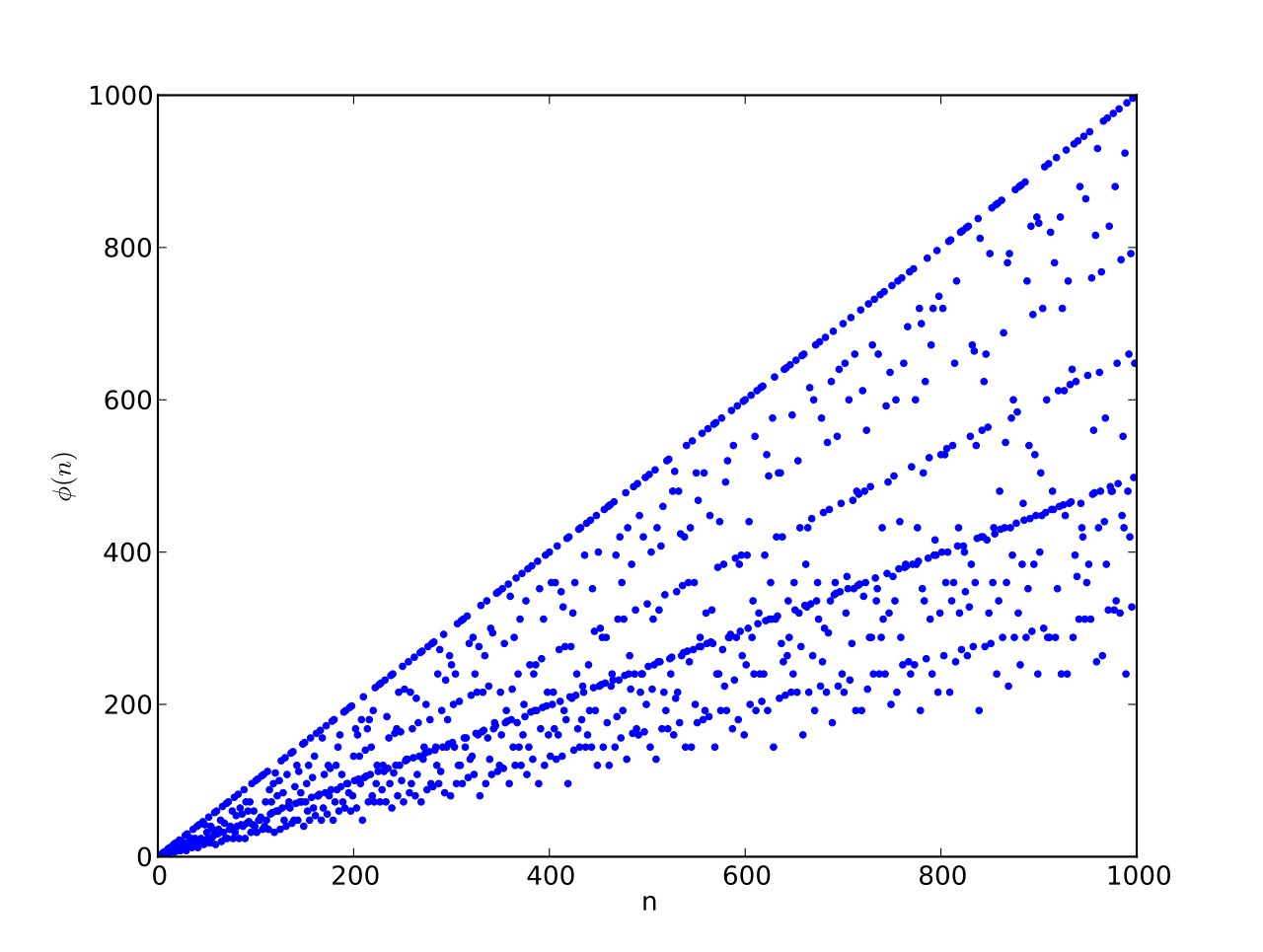
As you can see, eulerphi(n) = n-1 for primes. Now you know what the top line of the Eulerphi graph is. It’s the primes. Here’s a bigger version of the graph:

Graph of eulerphi(n) = φ(n)


Unlike the Ulam spiral, however, the Eulerphi graph is cramped. But it’s easy to stretch it. You can represent φ(n) as a fraction between 0 and 1 like this: phifrac(n) = φ(n) / (n-1). Using phifrac(n), you can create Eulerphi bands, like this:

Eulerphi band, n <= 1781


Eulerphi band, n <= 3561


Eulerphi band, n <= 7121


Eulerphi band, n <= 14241


Or you can create Eulerphi discs, like this:

Eulerphi disc, n <= 1601


Eulerphi disc, n <= 3201


Eulerphi disc, n <= 6401


Eulerphi disc, n <= 12802


Eulerphi disc, n <= 25602


But what is the bottom line of the Eulerphi bands and inner ring of the Eulerphi discs, where φ(n) is smallest relative to n? Well, the top line or outer ring is the primes and the bottom line or inner ring is the primorials (and their multiples). The function primorial(n) is the multiple of the first n primes:

primorial(1) = 2
primorial(2) = 2*3 = 6
primorial(3) = 2*3*5 = 30
primorial(4) = 2*3*5*7 = 210
primorial(5) = 2*3*5*7*11 = 2310
primorial(6) = 2*3*5*7*11*13 = 30030
primorial(7) = 2*3*5*7*11*13*17 = 510510
primorial(8) = 2*3*5*7*11*13*17*19 = 9699690
primorial(9) = 2*3*5*7*11*13*17*19*23 = 223092870
primorial(10) = 2*3*5*7*11*13*17*19*23*29 = 6469693230


Here are the numbers returning record lows for φfrac(n) = φ(n) / (n-1):

φ(4) = 2 (2/3 = 0.666…)
4 = 2^2
φ(6) = 2 (2/5 = 0.4)
6 = 2.3
φ(12) = 4 (4/11 = 0.363636…)
12 = 2^2.3
[…]
φ(30) = 8 (8/29 = 0.275862…)
30 = 2.3.5
φ(60) = 16 (16/59 = 0.27118…)
60 = 2^2.3.5
[…]
φ(210) = 48 (48/209 = 0.229665…)
210 = 2.3.5.7
φ(420) = 96 (96/419 = 0.2291169…)
420 = 2^2.3.5.7
φ(630) = 144 (144/629 = 0.228934…)
630 = 2.3^2.5.7
[…]
φ(2310) = 480 (480/2309 = 0.2078822…)
2310 = 2.3.5.7.11
φ(4620) = 960 (960/4619 = 0.20783719…)
4620 = 2^2.3.5.7.11
[…]
30030 = 2.3.5.7.11.13
φ(60060) = 11520 (11520/60059 = 0.191811385…)
60060 = 2^2.3.5.7.11.13
φ(90090) = 17280 (17280/90089 = 0.1918103209…)
90090 = 2.3^2.5.7.11.13
[…]
φ(510510) = 92160 (92160/510509 = 0.18052571061…)
510510 = 2.3.5.7.11.13.17
φ(1021020) = 184320 (184320/1021019 = 0.18052553…)
1021020 = 2^2.3.5.7.11.13.17
φ(1531530) = 276480 (276480/1531529 = 0.180525474868579…)
1531530 = 2.3^2.5.7.11.13.17
φ(2042040) = 368640 (368640/2042039 = 0.18052544540040616…)
2042040 = 2^3.3.5.7.11.13.17

Bi-Bell Basics

Here’s what you might call a Sisyphean sequence. It struggles upward, then slips back, over and over again:

1, 1, 2, 1, 2, 2, 3, 1, 2, 2, 3, 2, 3, 3, 4, 1, 2, 2, 3, 2, 3, 3, 4, 2, 3, 3, 4, 3, 4, 4, 5, 1, 2, 2, 3, 2, 3, 3, 4, 2, 3, 3, 4, 3, 4, 4, 5, 2, 3, 3, 4, 3, 4, 4, 5, 3, 4, 4, 5, 4, 5, 5, 6, 1, 2, 2, 3, 2, 3, 3, 4, 2, 3, 3, 4, 3, 4, 4, 5, 2, 3, 3, 4, 3, 4, 4, 5, 3, 4, 4, 5, 4, 5, 5, 6, 2, 3, 3, 4, 3, 4, 4, 5, 3, 4, 4, 5, 4, 5, 5, 6, 3, 4, 4, 5, 4, 5, 5, 6, 4, 5, 5, 6, 5, 6, 6, 7, 1, 2, 2, 3, 2, 3, 3, 4, 2...


The struggle goes on for ever. Every time it reaches a new maximum, it will fall back to 1 at the next step. And in fact 1, 2, 3 and all other integers occur infinitely often in the sequence, because it represents the digit-sums of binary numbers:

1 ← 1
1 = 1+0 ← 10 in binary = 2 in base ten
2 = 1+1 ← 11 = 3
1 = 1+0+0 ← 100 = 4
2 = 1+0+1 ← 101 = 5
2 = 1+1+0 ← 110 = 6
3 = 1+1+1 ← 111 = 7
1 = 1+0+0+0 ← 1000 = 8
2 = 1+0+0+1 ← 1001 = 9
2 = 1+0+1+0 ← 1010 = 10
3 = 1+0+1+1 ← 1011 = 11
2 = 1+1+0+0 ← 1100 = 12
3 = 1+1+0+1 ← 1101 = 13
3 = 1+1+1+0 ← 1110 = 14
4 = 1+1+1+1 ← 1111 = 15
1 = 1+0+0+0+0 ← 10000 = 16
2 = 1+0+0+0+1 ← 10001 = 17
2 = 1+0+0+1+0 ← 10010 = 18
3 = 1+0+0+1+1 ← 10011 = 19
2 = 1+0+1+0+0 ← 10100 = 20


Now here’s a related sequence in which all integers do not occur infinitely often:

1, 2, 3, 3, 4, 5, 6, 4, 5, 6, 7, 7, 8, 9, 10, 5, 6, 7, 8, 8, 9, 10, 11, 9, 10, 11, 12, 12, 13, 14, 15, 6, 7, 8, 9, 9, 10, 11, 12, 10, 11, 12, 13, 13, 14, 15, 16, 11, 12, 13, 14, 14, 15, 16, 17, 15, 16, 17, 18, 18, 19, 20, 21, 7, 8, 9, 10, 10, 11, 12, 13, 11, 12, 13, 14, 14, 15, 16, 17, 12, 13, 14, 15, 15, 16, 17, 18, 16, 17, 18, 19, 19, 20, 21, 22, 13, 14, 15, 16, 16, 17, 18, 19, 17, 18, 19, 20, 20, 21, 22, 23, 18, 19, 20, 21, 21, 22, 23, 24, 22, 23, 24, 25, 25, 26, 27, 28, 8, 9, 10, 11, 11, 12, 13, 14, 12, 13, 14, 15, 15...


The sequence represents the sum of the values of occupied columns in the binary numbers, reading from right to left:

10 in binary = 2 in base ten
21 (column values from right to left)
2*1 + 1*0 = 2


11 = 3
21
2*1 + 1*1 = 3


100 = 4
321 (column values from right to left)
3*1 + 2*0 + 1*0 = 3


101 = 5
321
3*1 + 2*0 + 1*1 = 4


110 = 6
321
3*1 + 2*1 + 1*0 = 5


111 = 7
321
3*1 + 2*1 + 1*1 = 6


1000 = 8
4321
4*1 + 3*0 + 2*0 + 1*0 = 4


1001 = 9
4321
4*1 + 3*0 + 2*0 + 1*1 = 5


1010 = 10
4321
4*1 + 3*0 + 2*1 + 1*0 = 6


1011 = 11
4321
4*1 + 3*0 + 2*1 + 1*1 = 7


1100 = 12
4321
4*1 + 3*1 + 2*0 + 1*0 = 7


1101 = 13
4321
4*1 + 3*1 + 2*0 + 1*1 = 8


1110 = 14
4321
4*1 + 3*1 + 2*1 + 1*0 = 9


1111 = 15
4321
4*1 + 3*1 + 2*1 + 1*1 = 10


10000 = 16
54321
5*1 + 4*0 + 3*0 + 2*0 + 1*0 = 5


In that sequence, although no number occurs infinitely often, some numbers occur more often than others. If you represent the count of sums up to a certain digit-length as a graph, you get a famous shape:

Bell curve formed by the count of column-sums in base 2


Bi-bell curves for 1 to 16 binary digits (animated)


In “Pi in the Bi”, I looked at that way of forming the bell curve and called it the bi-bell curve. Now I want to go further. Suppose that you assign varying values to the columns and try other bases. For example, what happens if you assign the values 2^p + 1 to the columns, reading from right to left, then use base 3 to generate the sums? These are the values of 2^p + 1:

2, 3, 5, 9, 17, 33, 65, 129, 257, 513, 1025...


And here’s an example of how you generate a column-sum in base 3:

2102 in base 3 = 65 in base ten
9532 (column values from right to left)
2*9 + 1*5 + 0*3 + 2*2 = 27


The graphs for these column-sums using base 3 look like this as the digit-length rises. They’re no longer bell-curves (and please note that widths and heights have been normalized so that all graphs fit the same space):

Graph for the count of column-sums in base 3 using 2^p + 1 (digit-length <= 7)

(width and height are normalized)


Graph for base 3 and 2^p + 1 (dl<=8)


Graph for base 3 and 2^p + 1 (dl<=9)


Graph for base 3 and 2^p + 1 (dl<=10)


Graph for base 3 and 2^p + 1 (dl<=11)


Graph for base 3 and 2^p + 1 (dl<=12)


Graph for base 3 and 2^p + 1 (animated)


Now try base 3 and column-values of 2^p + 2 = 3, 4, 6, 10, 18, 34, 66, 130, 258, 514, 1026…

Graph for base 3 and 2^p + 2 (dl<=7)


Graph for base 3 and 2^p + 2 (dl<=8)


Graph for base 3 and 2^p + 2 (dl<=9)


Graph for base 3 and 2^p + 2 (dl<=10)


Graph for base 3 and 2^p + 2 (animated)


Now try base 5 and 2^p + 1 for the columns. The original bell curve has become like a fractal called the blancmange curve:

Graph for base 5 and 2^p + 1 (dl<=7)


Graph for base 5 and 2^p + 1 (dl<=8)


Graph for base 5 and 2^p + 1 (dl<=9)


Graph for base 5 and 2^p + 1 (dl<=10)


Graph for base 5 and 2^p + 1 (animated)


And finally, return to base 2 and try the Fibonacci numbers for the columns:

Graph for base 2 and Fibonacci numbers = 1,1,2,3,5… (dl<=7)


Graph for base 2 and Fibonacci numbers (dl<=9)


Graph for base 2 and Fibonacci numbers (dl<=11)


Graph for base 2 and Fibonacci numbers (dl<=13)


Graph for base 2 and Fibonacci numbers (dl<=15)


Graph for base 2 and Fibonacci numbers (animated)


Previously Pre-Posted…

Pi in the Bi — bell curves generated by binary digits

Match of the Day

Some interesting shapes are mentioned in Derrick Niederman’s Number Freak (2010). Using identical matchsticks, what’s the smallest fully connected shape you can make in which two matches meet at every vertex? That is, what is the smallest 2-regular matchstick graph?

It’s an equilateral triangle:

2match

Now, what is the smallest fully connected shape you can make in which three matches meet at every vertex? That is, what is the smallest 3-regular matchstick graph? It uses twelve identical matches and looks like this:

3match

And here is the smallest known 4-regular matchstick graph, discovered by the German mathematician Heiko Harborth and using 104 identical matches:

4match

But Niederman says that “it’s impossible to create any arrangement in which five or more matchsticks meet at every vertex” (entry for “104”, pg. 230 of the 2012 paperback).

Pest Test

Health warning: I am not a mathematician. That said, here is a mathematical question:

Suppose there is a 99% accurate test for a medical condition – say a symptomless infection. You take the test and get a positive result. What are your chances of having the infection?

That obvious answer might seem to be 99%. But the obvious answer is wrong. The accuracy of the test is only half the information you need to answer the question. You also need to know how common the infection is. Say it occurs once in every hundred people. On average, then, if you test a hundred people, one of whom has the infection, you will get two positive results: one that is accurate and one that is inaccurate, i.e., a false positive. Under those circumstances, a positive result means that you have a ½, or 50%, chance of having the infection (see appendix for further discussion). Under some other circumstances, a positive result on an 80% or 90% accurate test would mean that you have a higher chance of having the infection. Here’s a graphic to illustrate this apparent paradox:

Graph illustrating confidence rates for medical tests of various accuracy

The x-axis represents infection rate per 10,000 of the population, the y-axis represents one’s chance of being infected, from 0%, for no chance, to 100%, for complete certainty. The coloured curves represent tests of different accuracy: 1% accurate, for the bottom curve, and 99% accurate, for the uppermost curve. The curves between the two represent tests of 10% to 90% accuracy. Note how the curves mirror each other: the 99% accurate test rises towards certainty very quickly, but takes a long time to finally get there. The 1% accurate test stays near complete uncertainty for a long time, then finally rises rapidly towards certainty. In other words, a positive result on a 99% accurate test is equivalent to a negative result on a 1% accurate test, and vice versa. Ditto for the 90% and 10% accurate tests, and so on. But a positive (or negative) result on a 50% accurate test is useless, because it never tells you anything new: your chance of being infected, given a positive result, is the same as the rate of infection in the population. And when exactly half the population is infected, your chance of being infected, given a positive result, is the same as the accuracy of the test, whether it’s 1%, 50%, or 99%.

Here is a table illustrating the same points:

Accuracy of test →


Infection rate ↓

1% 10% 20% 30% 40% 50% 60% 70% 80% 90% 99%
1/100 <1% 0.1% 0.3% 0.4% 0.7% 1% 1.5% 2.3% 3.9% 8.3% 50%
10/100 0.1% 1.2% 2.7% 4.5% 6.9% 10% 14.3% 20.6% 30.8% 50% 91.7%
20/100 0.3% 2.7% 5.9% 9.7% 14.3% 20% 27.3% 36.8% 50% 69.2% 96.1%
30/100 0.4% 4.5% 9.7% 15.5% 22.2% 30% 39.1% 50% 63.2% 79.4% 97.7%
40/100 0.7% 6.9% 14.3% 22.2% 30.8% 40% 50% 60.9% 72.7% 85.7% 98.5%
50/100 1% 10% 20% 30% 40% 50% 60% 70% 80% 90% 99%
60/100 1.5% 14.3% 27.3% 39.1% 50% 60% 69.2% 77.8% 85.7% 93.1% 99.3%
70/100 2.3% 20.6% 36.8% 50% 60.9% 70% 77.8% 84.5% 90.3% 95.5% 99.6%
80/100 3.9% 30.8% 50% 63.2% 72.7% 80% 85.7% 90.3% 94.1% 97.3% 99.7%
90/100 8.3% 50% 69.2% 79.4% 85.7% 90% 93.1% 95.5% 97.3% 98.8% 99.9%
99/100 50% 91.7% 96.1% 97.7% 98.5% 99% 99.3% 99.6% 99.7% 99.9% >99.9%
100/100 100% 100% 100% 100% 100% 100% 100% 100% 100% 100% 100%

Appendix

We’ve seen that we have to take false positives into account, but what about false negatives? Suppose that the rate of infection is 1 in 100 and the accuracy of the test is 99%. If the population is 10,000, then 100 people will have the disease and 9,900 will not. If the population is tested, on average 100 x 99% = 99 of the infected people will get an accurate positive result and 100 x 1% = 1 will get an inaccurate negative result, i.e., a false negative. Similarly, 9,900 x 1% = 99 of the non-infected people will get a false positive. So there will be 99 + 99 = 198 positive results, of which 99 are accurate. 99/198 = 1/2 = 50%.