Here’s a graph representing the fractional parts of √n for n = 1 to 1832, with frac(√1) at the top left and frac(√1832) at the bottom right:

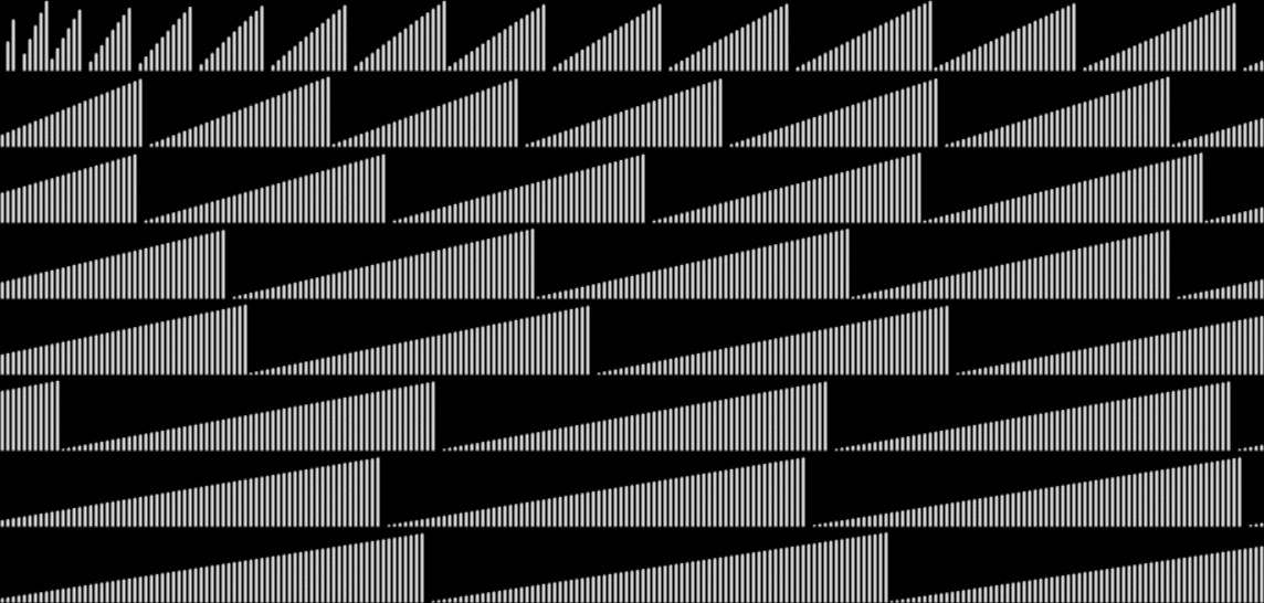
graph for frac(√n), n = 1..1832

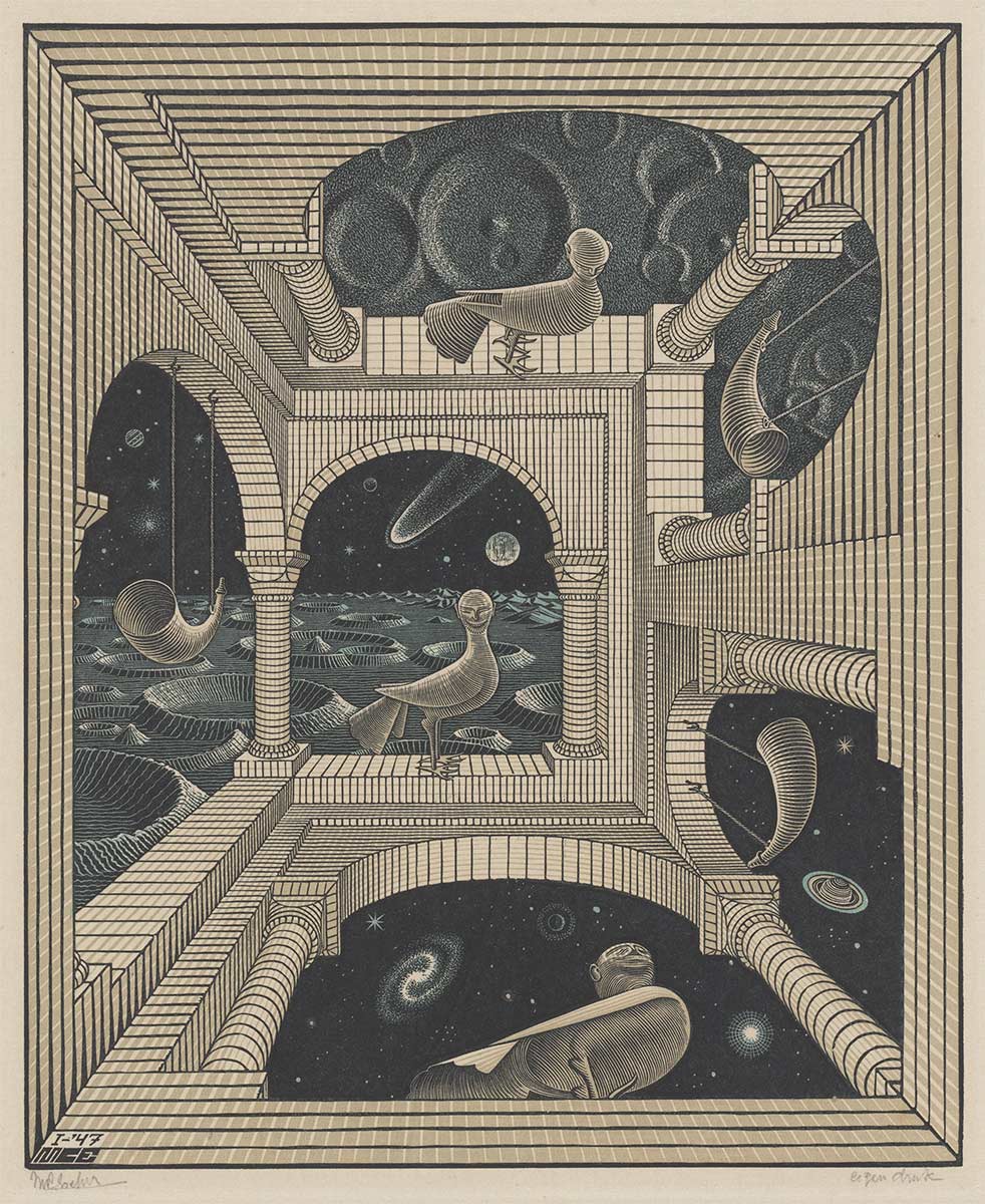
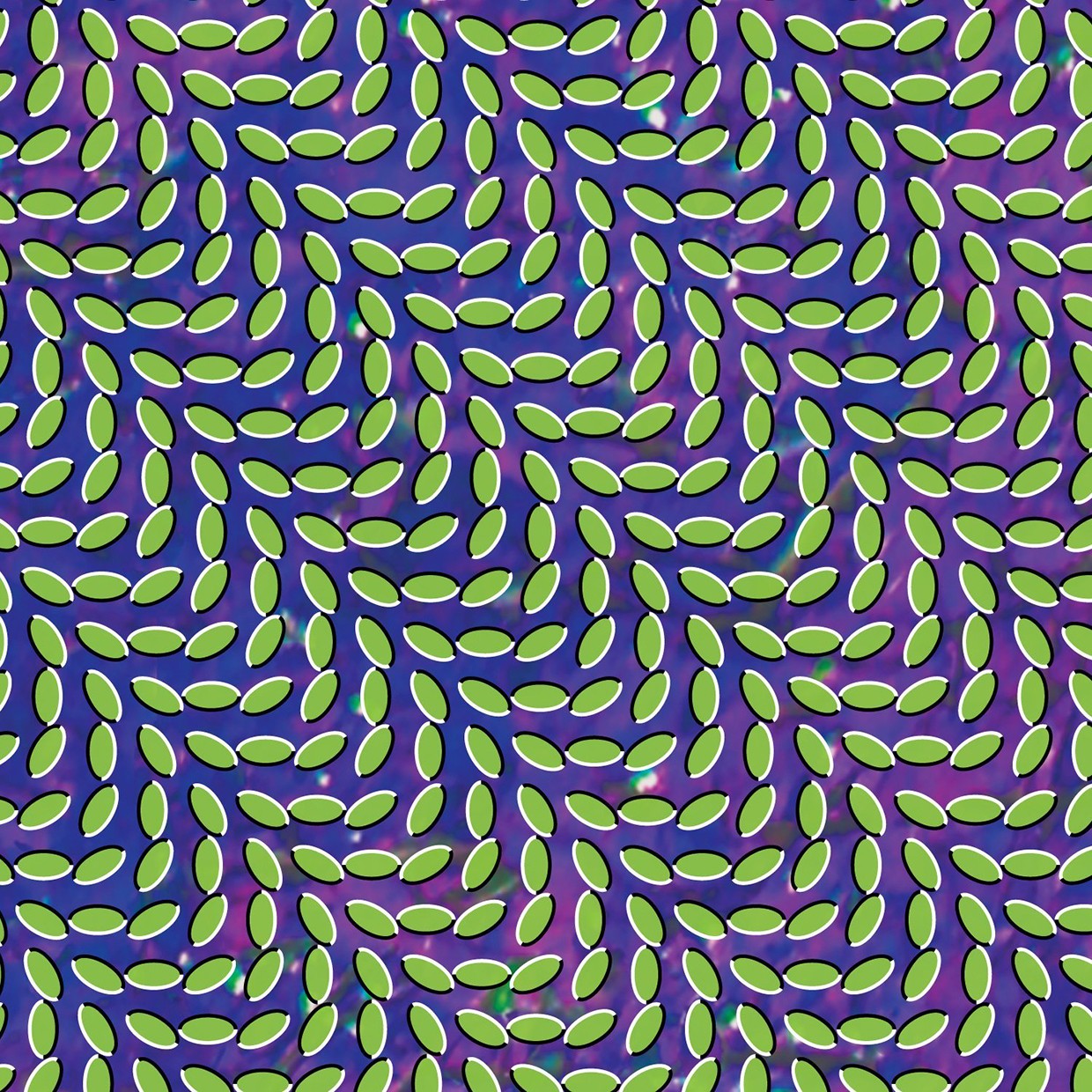
There’s an odd optical illusion making it seem as though each set of triangular waves ends lower on the right than it starts on the left. Otherwise, it’s a dull graph, because the fractional part of √n simply rises towards 0.9999…, then falls to 0 like this:

0 = frac(1) = frac(√1)
0.414213562373… = frac(1.414213562373…) = frac(√2)
0.732050807568… = frac(1.732050807568…) = frac(√3)
0 = frac(2) = frac(√4)
0.236067977499… = frac(2.236067977499…) = frac(√5)
0.449489742783… = frac(2.449489742783…) = frac(√6)
0.645751311064… = frac(2.645751311064…) = frac(√7)
0.828427124746… = frac(2.828427124746…) = frac(√8)
0 = frac(3) = frac(√9)
0.162277660168… = frac(3.162277660168…) = frac(√10)
0.316624790355… = frac(3.316624790355…) = frac(√11)
0.464101615137… = frac(3.464101615137…) = frac(√12)
0.605551275463… = frac(3.605551275463…) = frac(√13)
0.741657386773… = frac(3.741657386773…) = frac(√14)
0.872983346207… = frac(3.872983346207…) = frac(√15)
0 = frac(4) = frac(√16)
0.123105625617… = frac(4.123105625617…) = frac(√17)
0.242640687119… = frac(4.242640687119…) = frac(√18)
0.358898943540… = frac(4.358898943540…) = frac(√19)
0.472135954999… = frac(4.472135954999…) = frac(√20)

But what about the fractional parts of the sum of √n? What does that graph look like? Much more interesting:

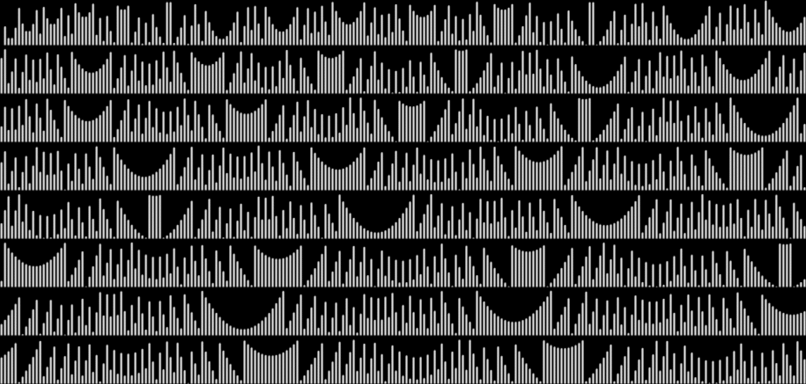
frac(sum(√n)), n = 1..1832

Here are the fractional parts for the sum of √n:

0 = frac(1) = frac(sum(√1))
0.414213562373… = frac(02.414213562373…) = frac(sum(√1..√2))
0.146264369941… = frac(04.146264369941…) = frac(sum(√1..√3))
0.146264369941… = frac(06.146264369941…) = frac(sum(√1..√4))
0.382332347441… = frac(08.382332347441…) = frac(sum(√1..√5))
0.831822090224… = frac(10.831822090224…) = frac(sum(√1..√6))
0.477573401289… = frac(13.477573401289…) = frac(sum(√1..√7))
0.306000526035… = frac(16.306000526035…) = frac(sum(√1..√8))
0.306000526035… = frac(19.306000526035…) = frac(sum(√1..√9))
0.468278186204… = frac(22.468278186204…) = frac(sum(√1..√10))
0.784902976559… = frac(25.784902976559…) = frac(sum(√1..√11))
0.249004591697… = frac(29.249004591697…) = frac(sum(√1..√12))
0.854555867161… = frac(32.854555867161…) = frac(sum(√1..√13))
0.596213253935… = frac(36.596213253935…) = frac(sum(√1..√14))
0.469196600142… = frac(40.469196600142…) = frac(sum(√1..√15))
0.469196600142… = frac(44.469196600142…) = frac(sum(√1..√16))
0.592302225760… = frac(48.592302225760…) = frac(sum(√1..√17))
0.834942912879… = frac(52.834942912879…) = frac(sum(√1..√18))
0.193841856420… = frac(57.193841856420…) = frac(sum(√1..√19))
0.665977811419… = frac(61.665977811419…) = frac(sum(√1..√20))

As with square roots, so with cube roots. The graph of frac(∛n) looks like this:

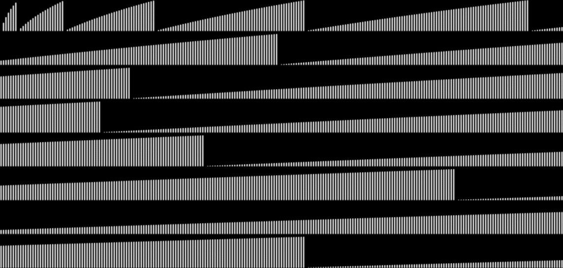
frac(∛n), n = 1..1832

It’s dull again, because the fractional part of ∛n is simply rising towards 0.9999…, then falling to 0. Just more slowly. But the graph of frac(sum(∛n)) looks like this:

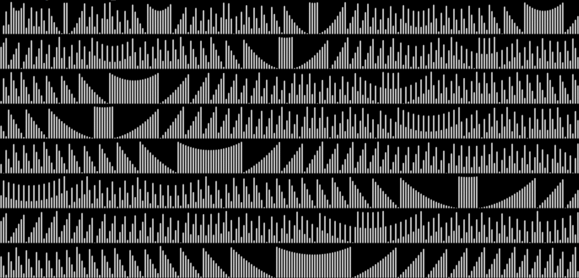
frac(sum(∛n))

But roots don’t end with √n and ∛n, of course. Those roots represent n^(1/2) and n^(1/3), respectively, because when x = n^(a/b), n = x^(b/a). What about the graph of sum(n^(4/5)), where n = (n^4/5)^(5/4)? The graph looks like this:

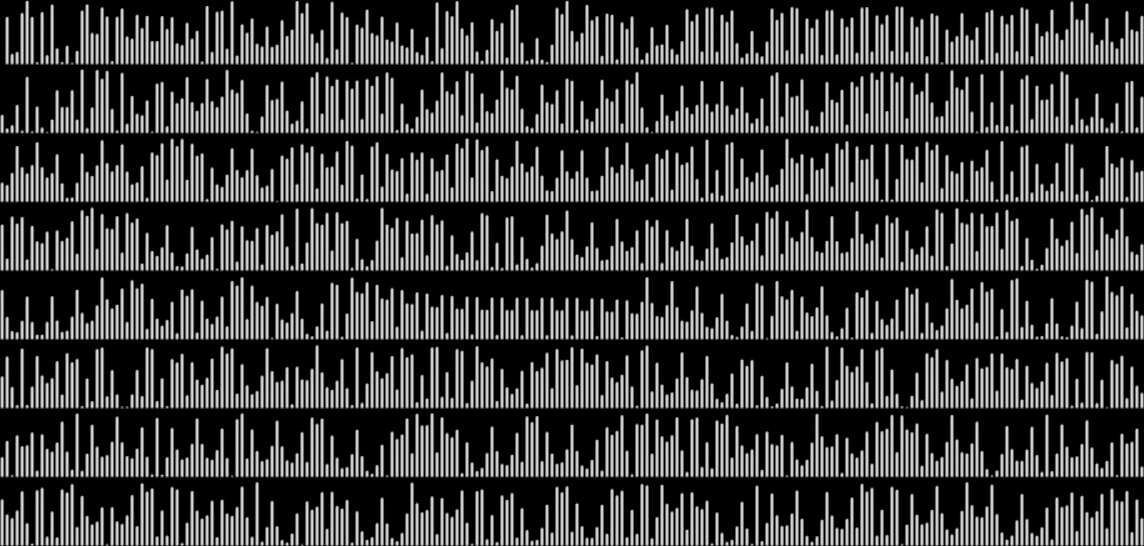
frac(sum(n^(4/5)))

One of the curves in that graph reminds of the cephalopodic tentacles in Jean Delville’s marvellous painting Les Trésors de Sathan (sic) (Treasures of Satan) (1895), which was used on the cover of Morbid Angel’s Blessed Are the Sick (1991). The curve is longer in frac(sum(n^(84/97))):

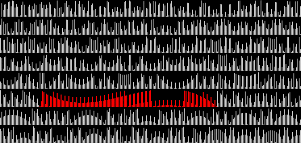
frac(sum(n^(84/97))) (curve in red)

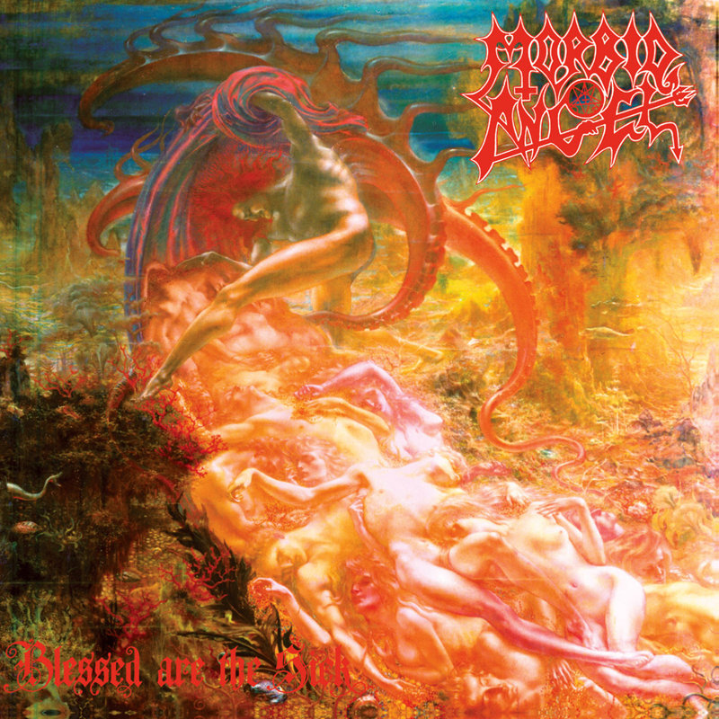
Les Trésors de Sathan (1895) by Jean Delville as the cover of Blessed Are the Sick (1991)

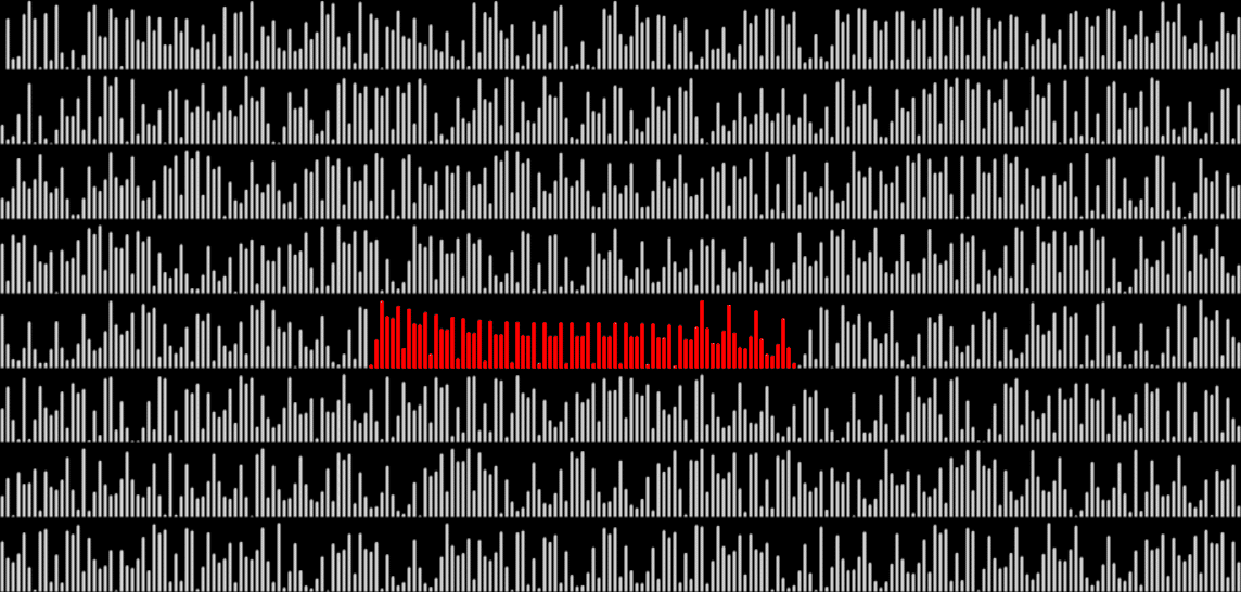
frac(sum(n^(4/5))) (curve in red)

Those Delvillean curves are examples of how, as the a/b of n^(a/b) climbs from 1/b to (b-1)/b, the graph of frac(sum(n^(a/b))) changes in interesting ways. Here are the graphs for n^(1..10/11):

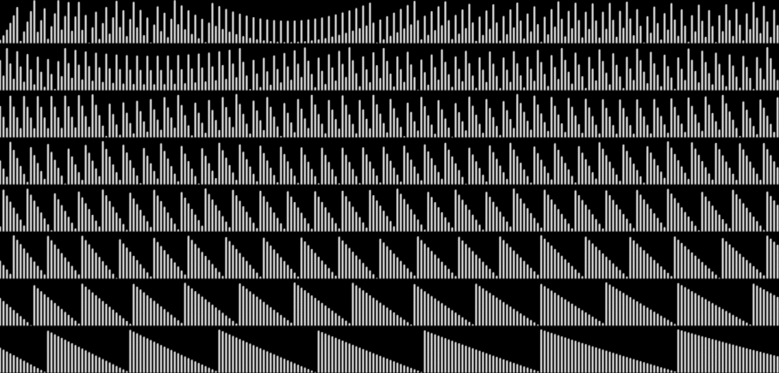
frac(sum(n^(1/11)))

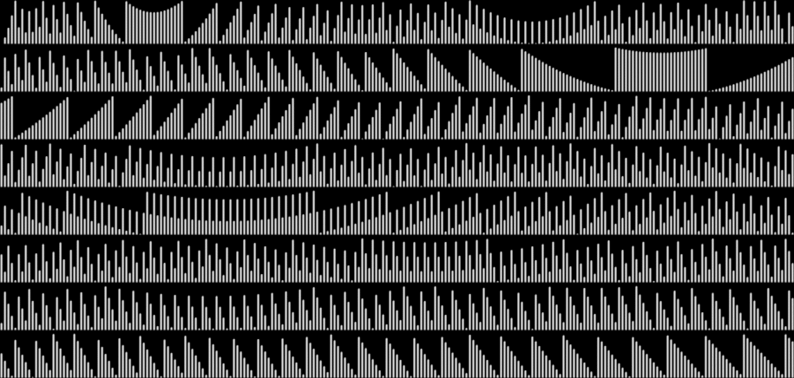
frac(sum(n^(2/11)))

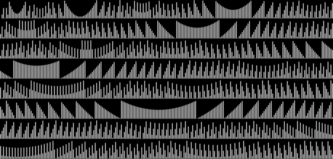
frac(sum(n^(3/11)))

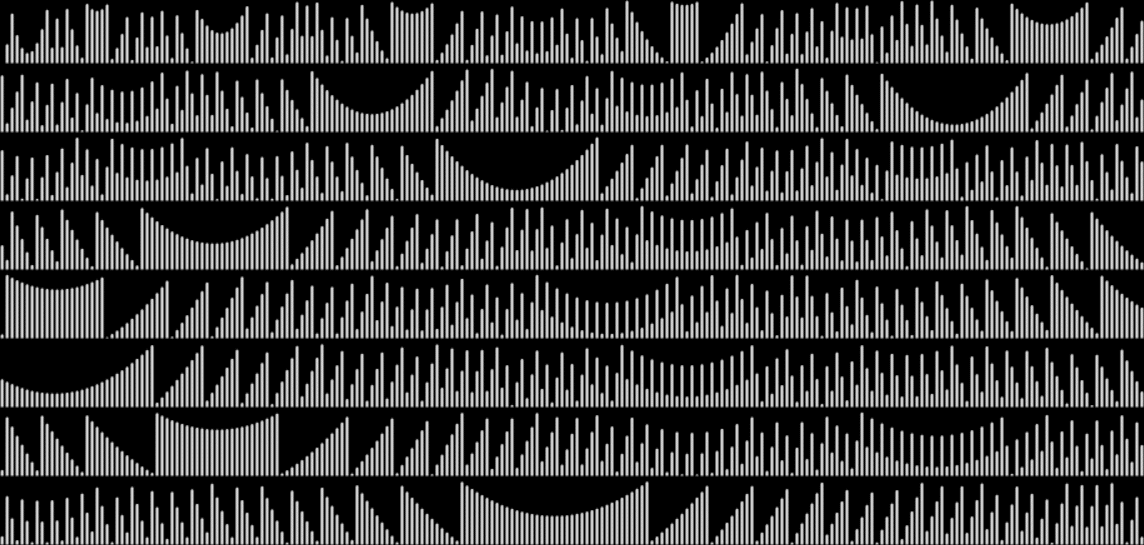
frac(sum(n^(4/11)))

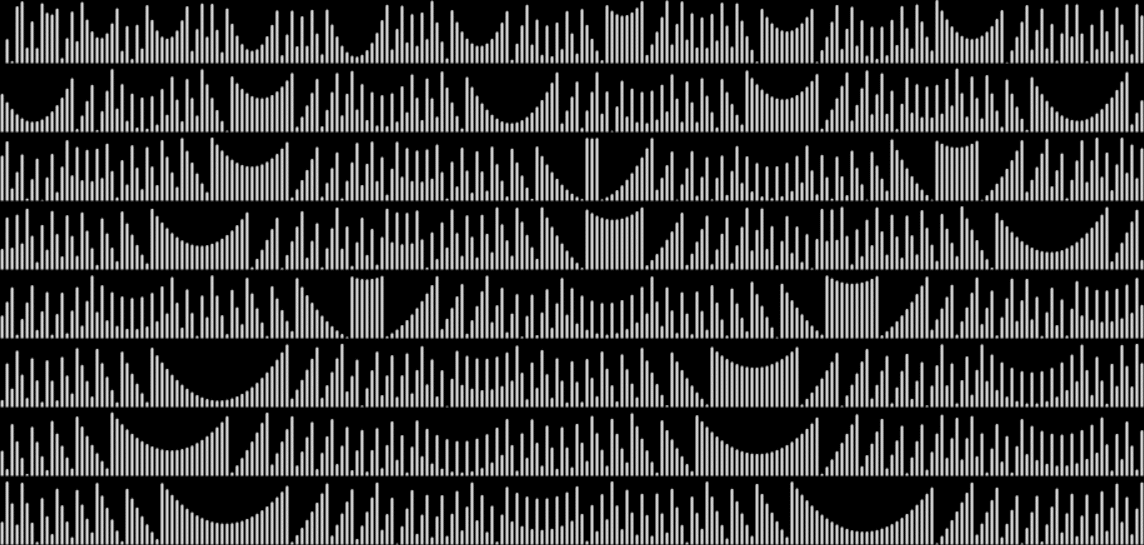
frac(sum(n^(5/11)))

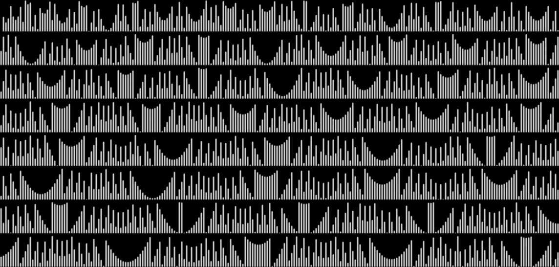
frac(sum(n^(6/11)))

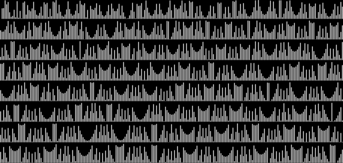
frac(sum(n^(7/11)))

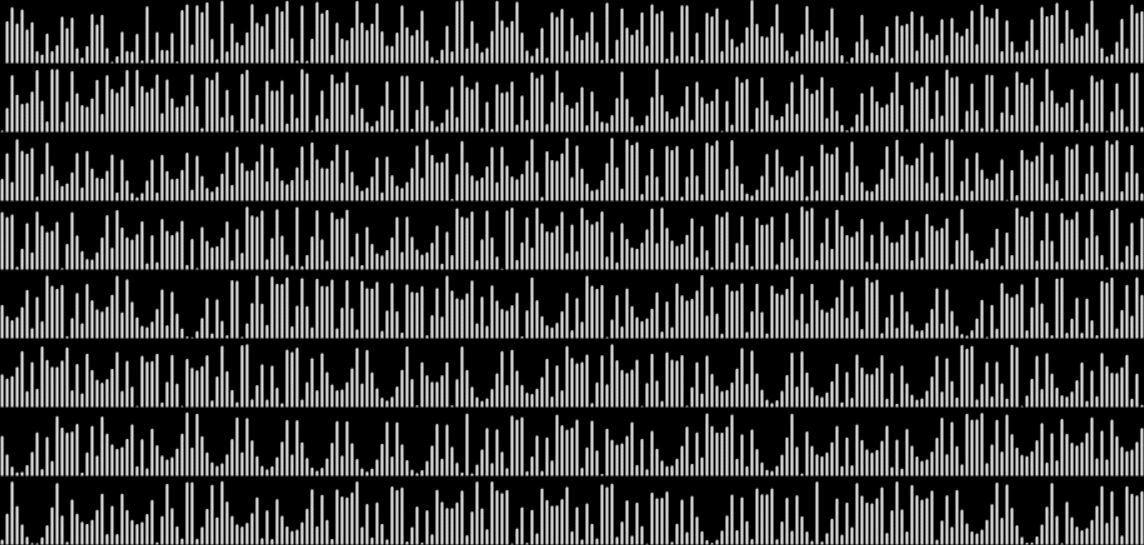
frac(sum(n^(8/11)))

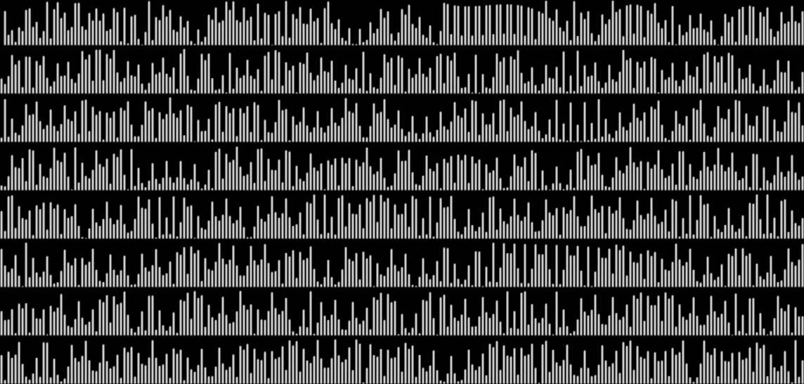
frac(sum(n^(9/11)))

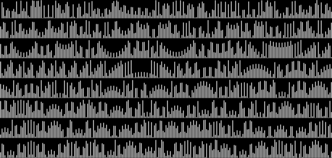
frac(sum(n^(10/11)))

Here’s an animation of those graphs:

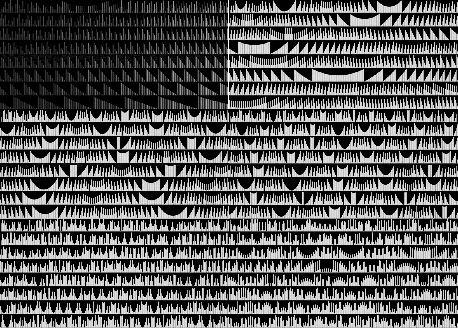
animation of frac(sum(n^(1/11..10/11))) (created at ezGif)

And here are graphs for n^(72/83) and n^(82/83), with a Delvillean curve in the graph of 72/83 and domes in the graph of 82/83:

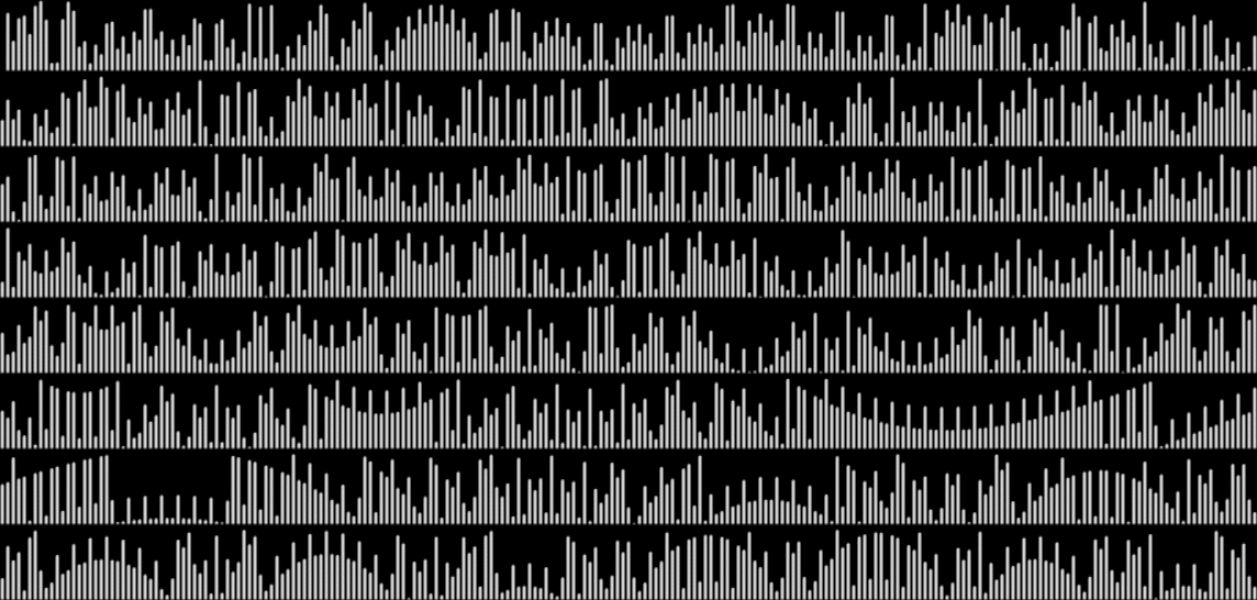
frac(sum(n^(72/83)))

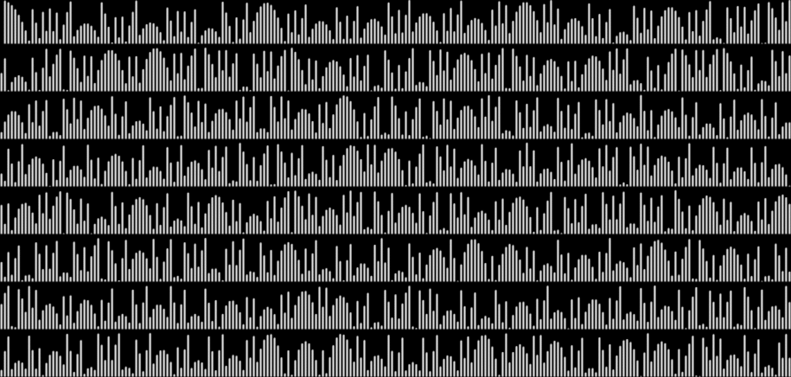
frac(sum(n^(82/83)))

As the denominators get bigger, so do the domes:

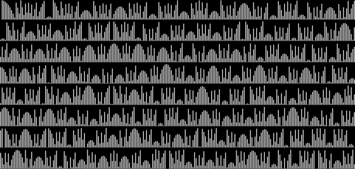
frac(sum(n^(1000/1009)))

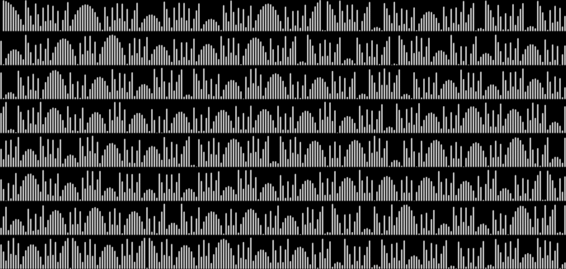
frac(sum(n^(1001/1009)))

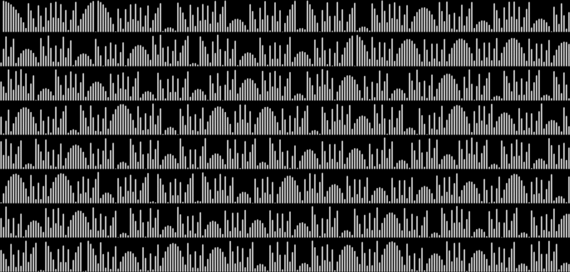
frac(sum(n^(1002/1009)))

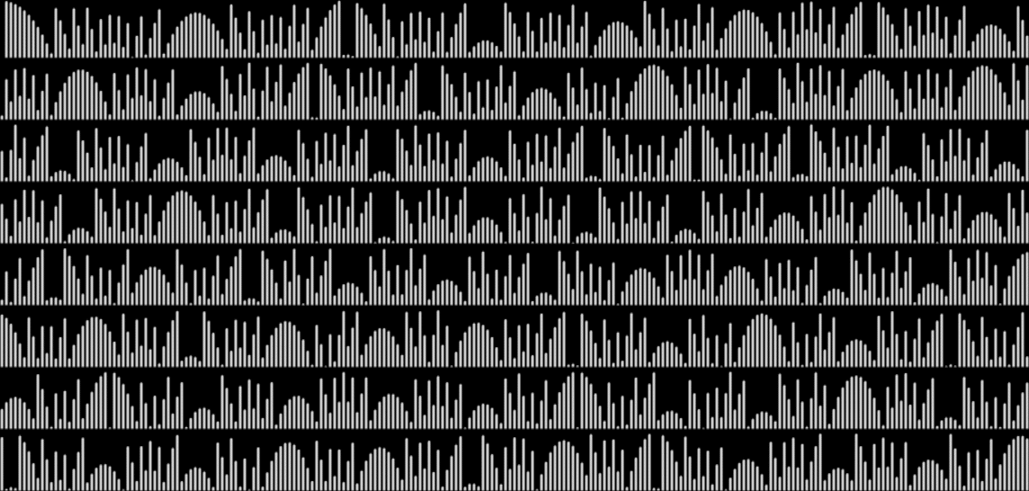
frac(sum(n^(1003/1009)))

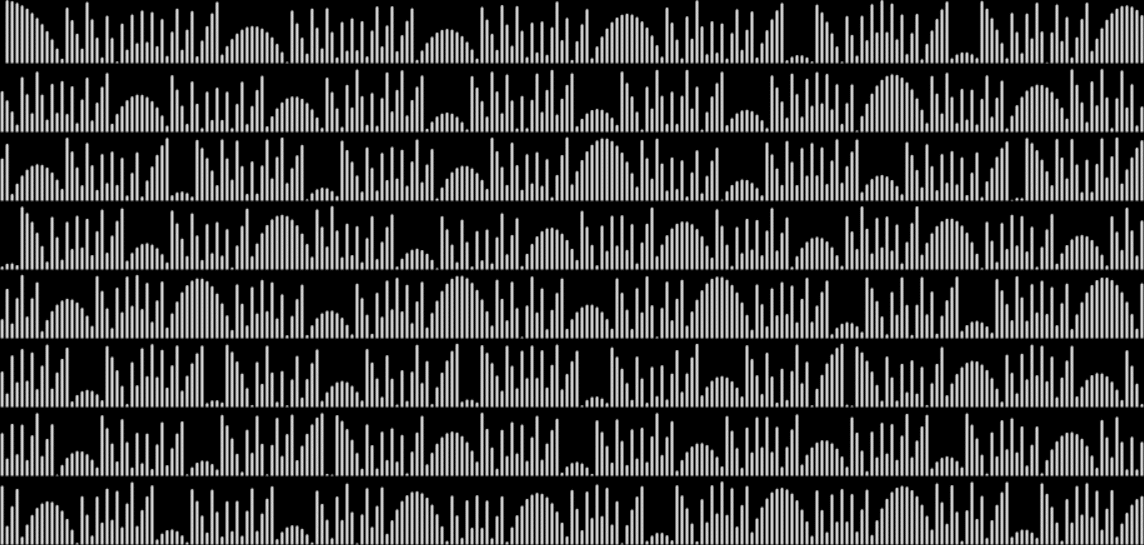
frac(sum(n^(1004/1009)))

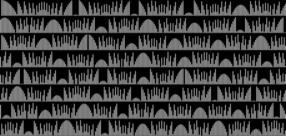
frac(sum(n^(1005/1009)))

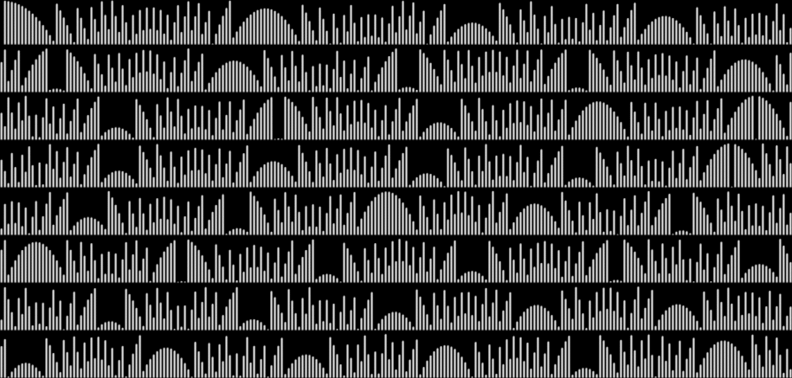
frac(sum(n^(1006/1009)))

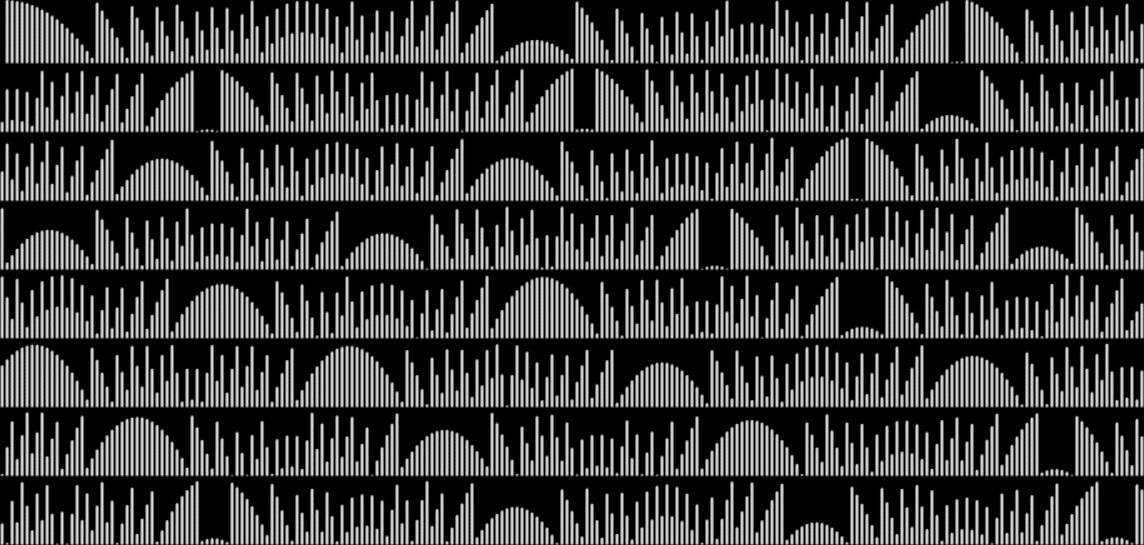
frac(sum(n^(1007/1009)))

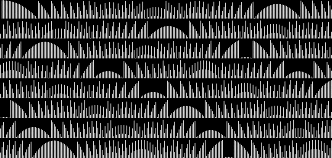
frac(sum(n^(1008/1009)))

Here’s an animation of those graphs:

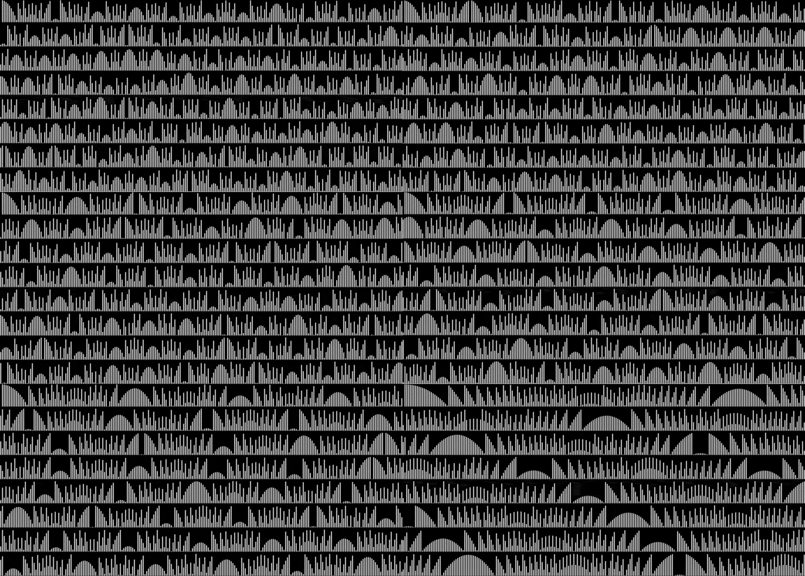
animation of frac(sum(n^(1000/1009..1008/1009))) (created at ezGif)

Previously Pre-Posted…

• Think Frinc — an earlier look at fraction-patterns
• Altars of Mathness — and similar patterns from integer-digits

Elsewhere Other-Accessible…

• Jean Delville at Wikipedia
• Blessed Are the Sick at BandCamp