What could be duller than digits? They just sit there on the page or screen, mindlessly marking mathematics:
1, 2, 3, 4, 5, 6, 7, 8, 9, 10, 11, 12, 13, 14, 15, 16, 17, 18, 19, 20, 21, 22, 23, 24, 25, 26, 27, 28, 29, 30, 31, 32, 33, 34, 35, 36, 37, 38, 39, 40, 41, 42, 43, 44, 45, 46, 47, 48, 49, 50, 51, 52, 53, 54, 55, 56, 57, 58, 59, 60, 61, 62, 63, 64, 65, 66, 67, 68, 69, 70, 71, 72, 73, 74, 75, 76, 77, 78, 79, 80, 81, 82, 83, 84, 85, 86, 87, 88, 89, 90, 91, 92, 93, 94, 95, 96, 97, 98, 99, 100…
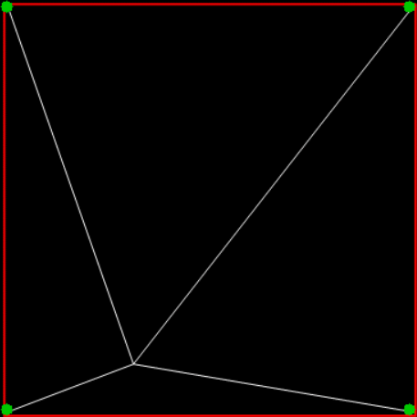
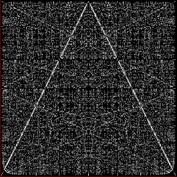
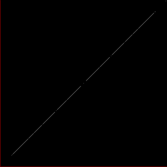
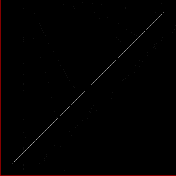
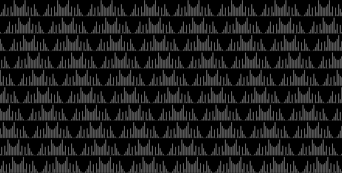
But perhaps they become more interesting as images. Let’s display the final digit of the integers, or counting numbers, on a graph. Running left-right and up-down, the graph represents the final or rightmost digit of 1, 2, 3, … 10, 11, 12, 13, … 100, 101, 102, 103, …, 1000, 1001, 1002, 1003, …:

Rightmost single digit of the integers (click for larger)
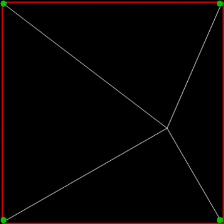
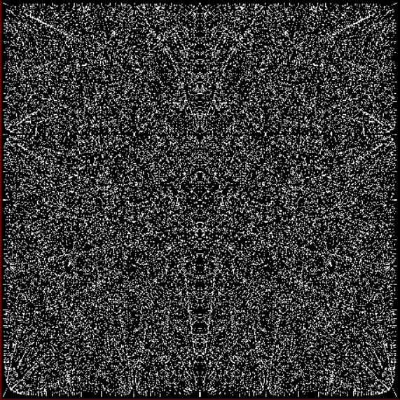
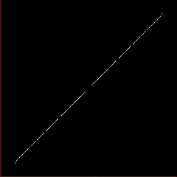
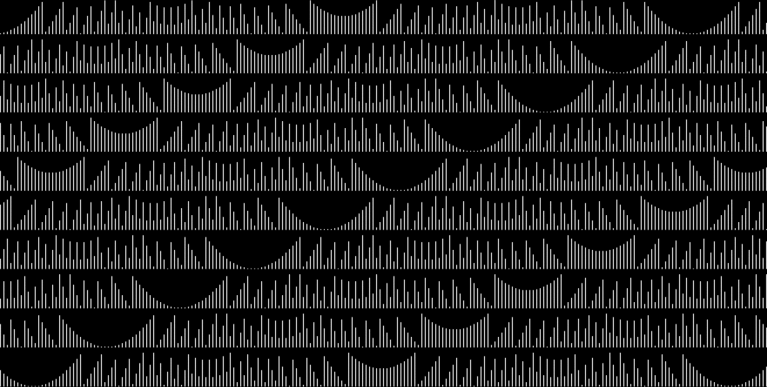
No, that’s still dull: the graph just generates endlessly repeating triangles. After all, the final digits fall into a cycle: 1, 2, 3, 4, 5, 6, 7, 8, 9, 0, 1, 2, 3… So do the final two digits: 1, 2, 3, 4, 5, […] 94, 95, 96, 97, 98, 99, 00, 01, 02, 03… Here they are as a graph:
Rightmost two digits of the integers
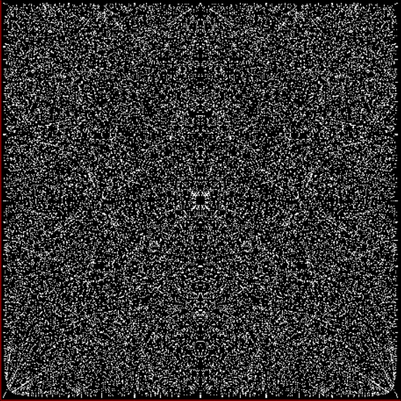
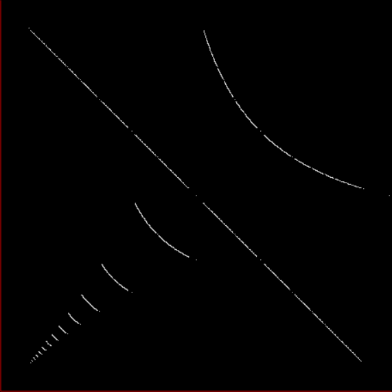
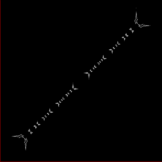
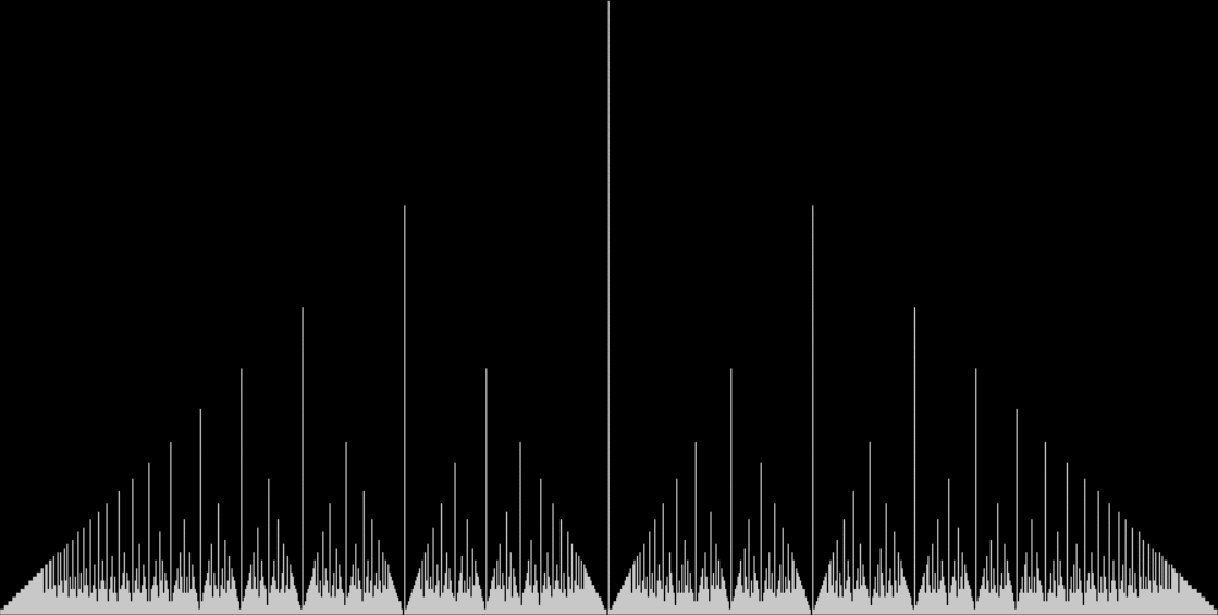
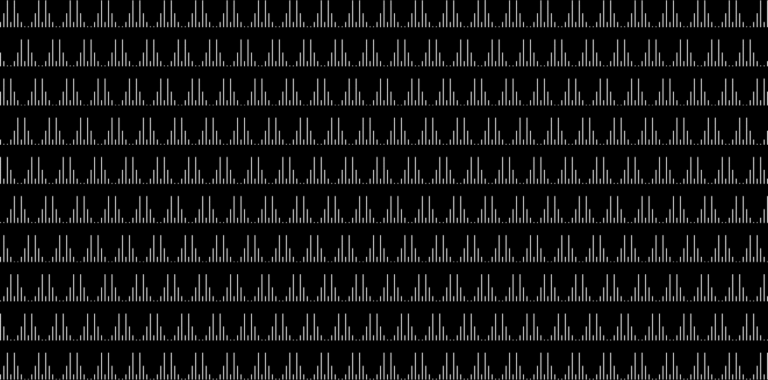
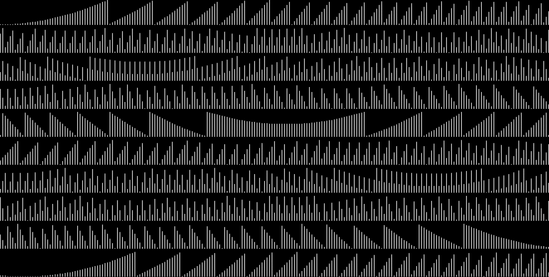
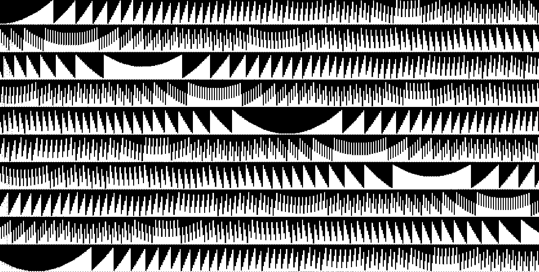
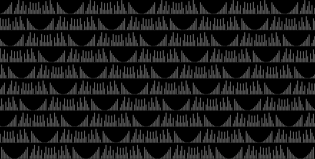
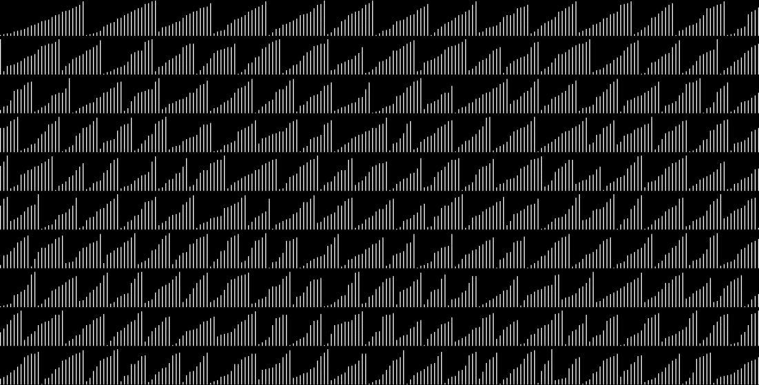
Now the triangles look like waves sweeping to shore. That’s a bit more interesting, but not much. So let’s try something different. The trailing digits of the integers generate triangles, so let’s see what the triangular numbers generate. The triangular numbers — 0, 1, 3, 6, 10, 15, 21… — are very simple to form. You just sum the integers: 1, 3 = 1 + 2, 6 = 1 + 2 + 3, 10 = 1 + 2 + 3 + 4, 15 = 1 + 2 + 3 + 4 + 5, 21 = 1 + 2 + 3 + 4 + 5 + 6, 28 = 1 + 2 + 3 + 4 + 5 + 6 + 7, 36 = 1 + 2 + 3 + 4 + 5 + 6 + 7 + 8, 45 = 1 + 2 + 3 + 4 + 5 + 6 + 7 + 8 + 9, 55 = 1 + 2 + 3 + 4 + 5 + 6 + 7 + 8 + 9 + 10… Here are the final digits of the triangulars — 1, 3, 6, 0, 5, 1, 8, 6… — as a graph:
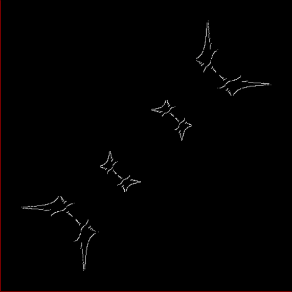
Final digit of triangular numbers in base 10 (click for larger)
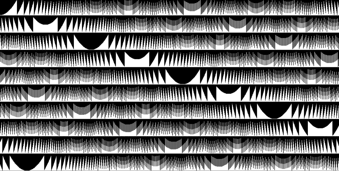
Now something interesting has appeared. The final digits form a repeated palindromic pattern (counting 0 as the zero-th triangular number):
0, 1, 3, 6, 0, 5, 1, 8, 6, 5, 5, 6, 8, 1, 5, 0, 6, 3, 1, 0, 0, 1, 3, 6, 0, 5, 1, 8, 6, 5, 5, 6, 8, 1, 5, 0, 6, 3, 1, 0, 0, 1, 3, 6, 0, 5, 1, 8, 6, 5, 5, 6, 8, 1, 5, 0, 6, 3, 1, 0, 0, 1, 3, 6, 0, 5, 1, 8, 6, 5, 5, 6, 8, 1, 5, 0, 6, 3, 1, 0, …
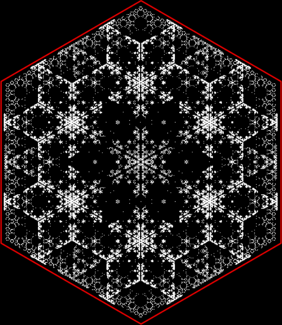
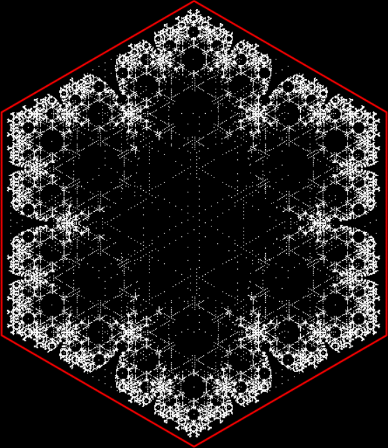
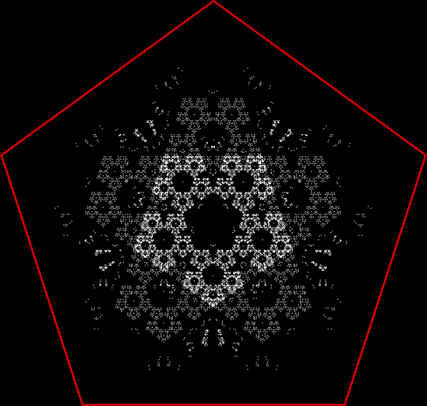
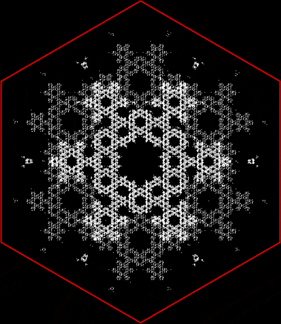
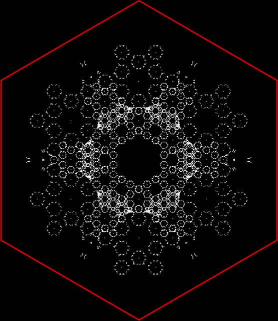
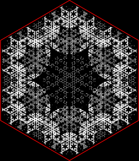
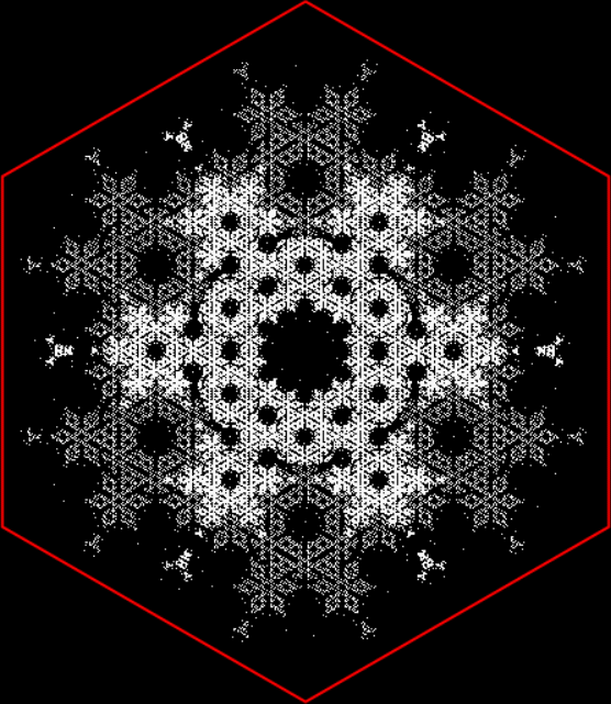
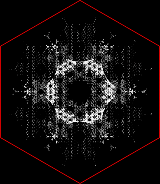
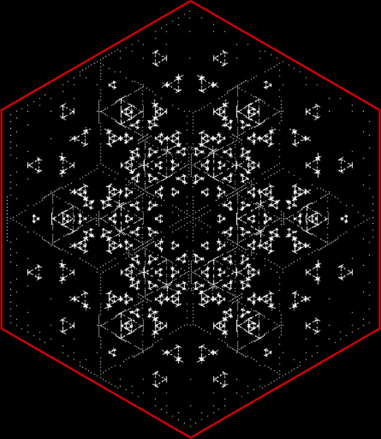
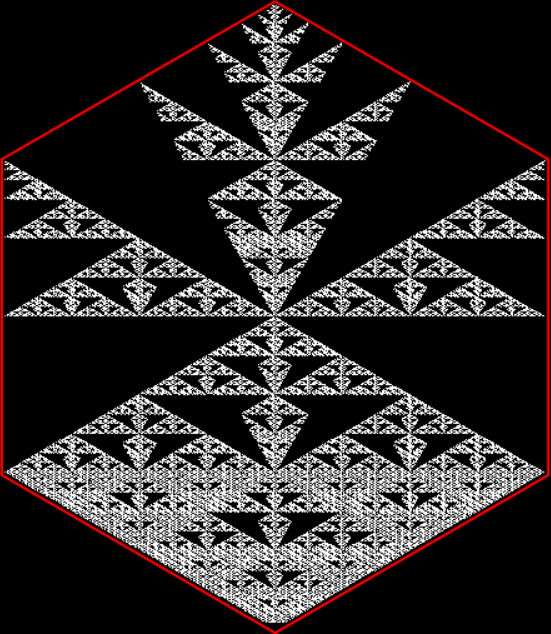
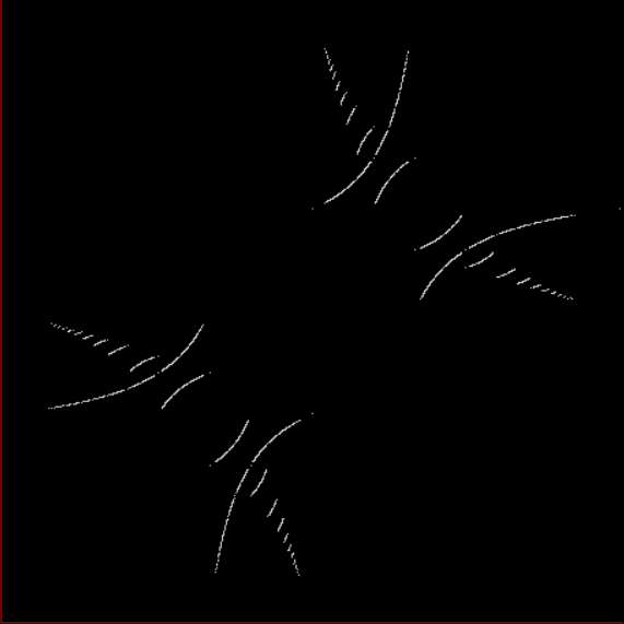
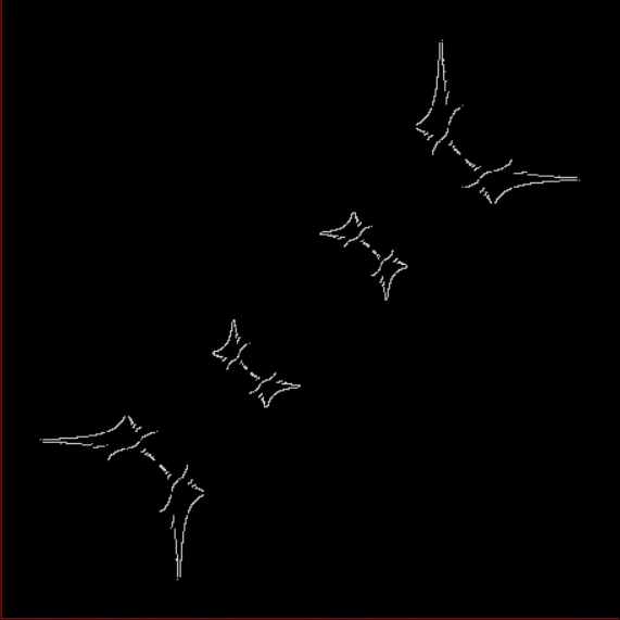
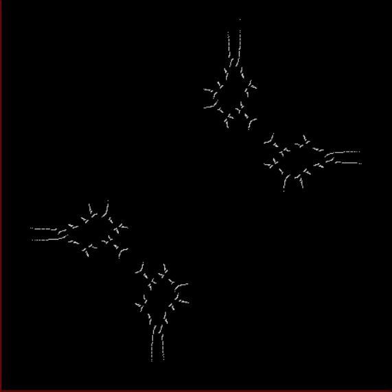
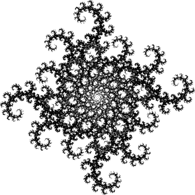
An Altar of Mathness created by the final digit of triangular numbers in base 10
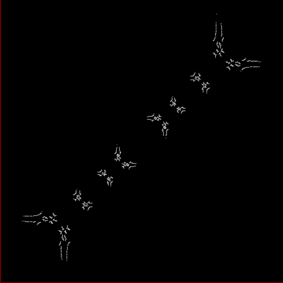
And those palindromic digits create symmetric shapes that remind me of little altars — let’s call them “altars of mathness” in tribute to Morbid Angel’s genre-defining album Altars of Madness (1989). And what about the final two digits of the triangular numbers? Here’s the graph (adjusted so that 99 fits into the same space as 9):

Final two digits of triangulars in b10
Final two triangular digits in b10 (horizontal scale compressed)
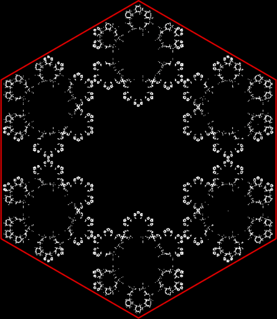
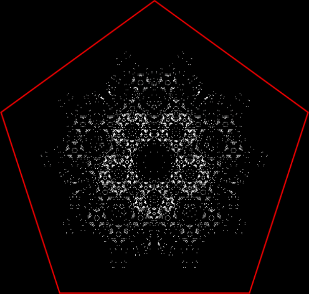
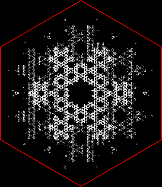
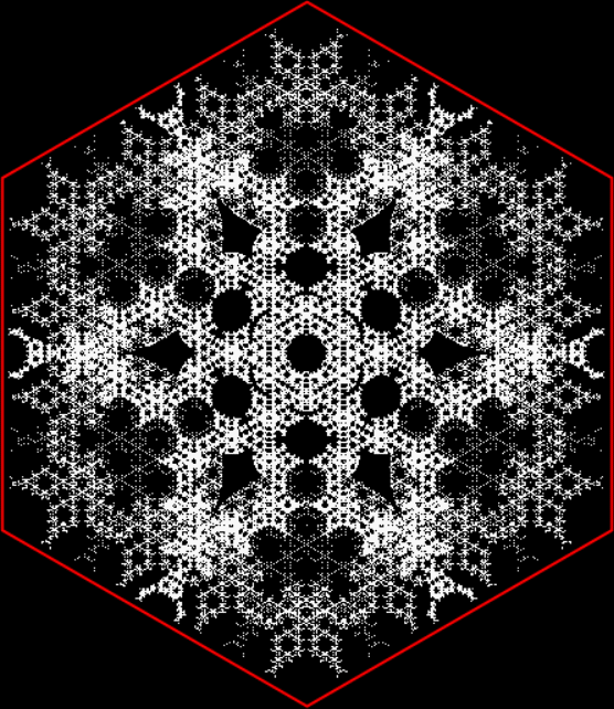
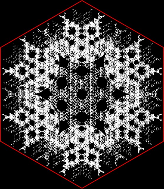
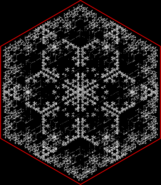
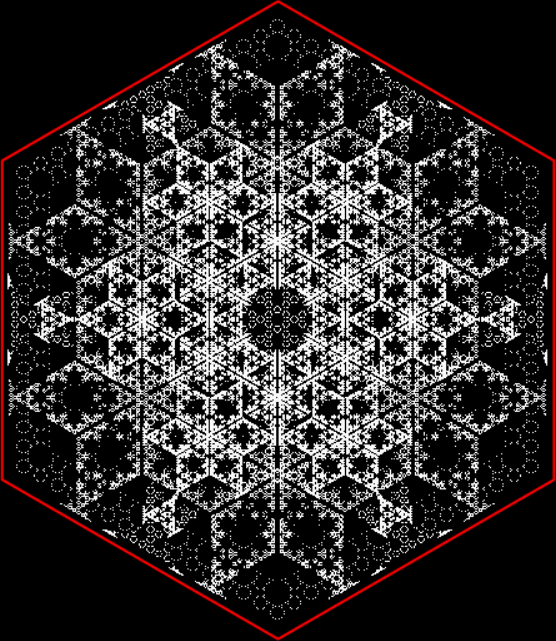
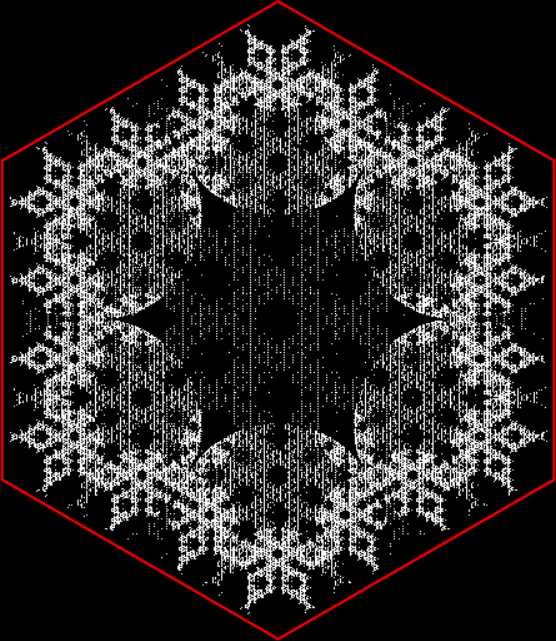
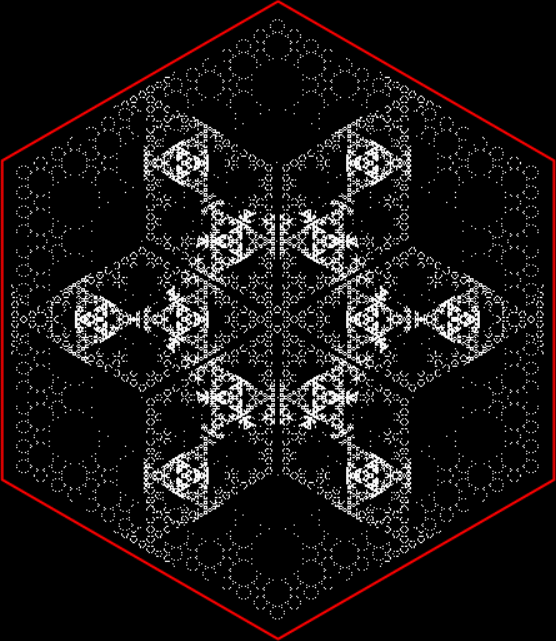
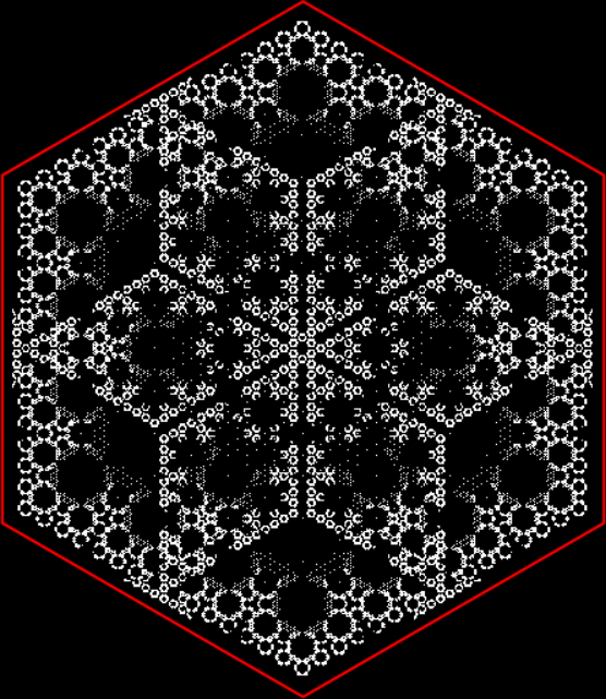
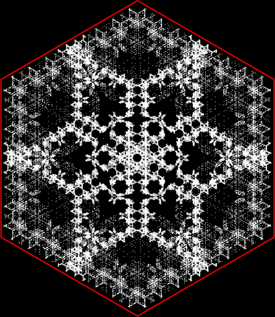
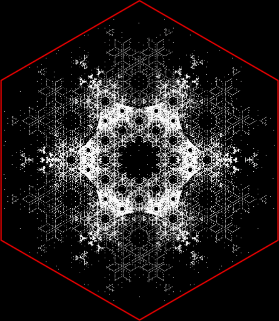
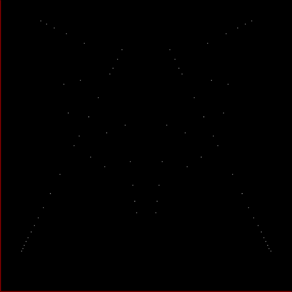
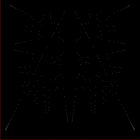
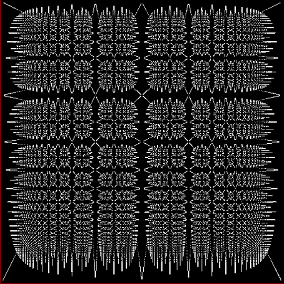
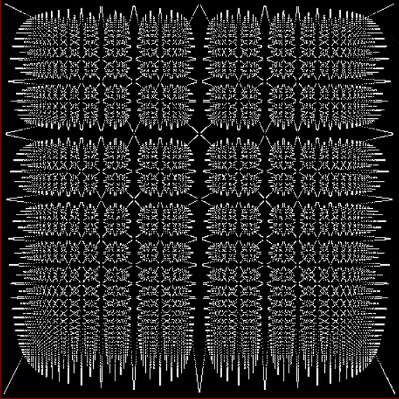
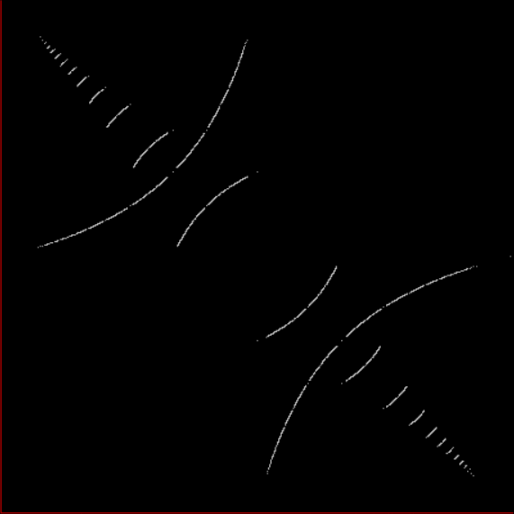
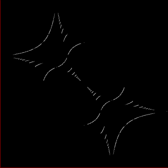
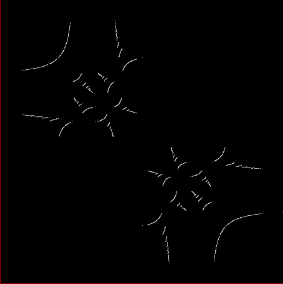
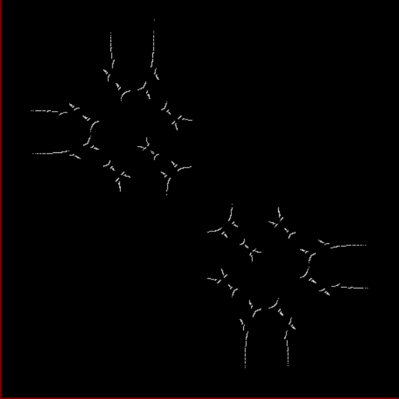
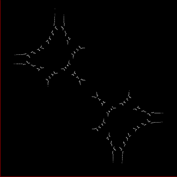
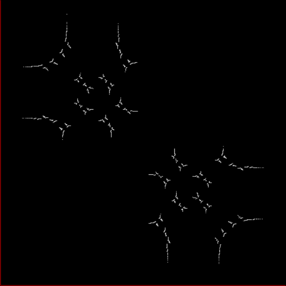
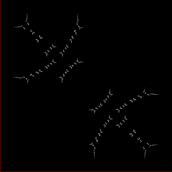
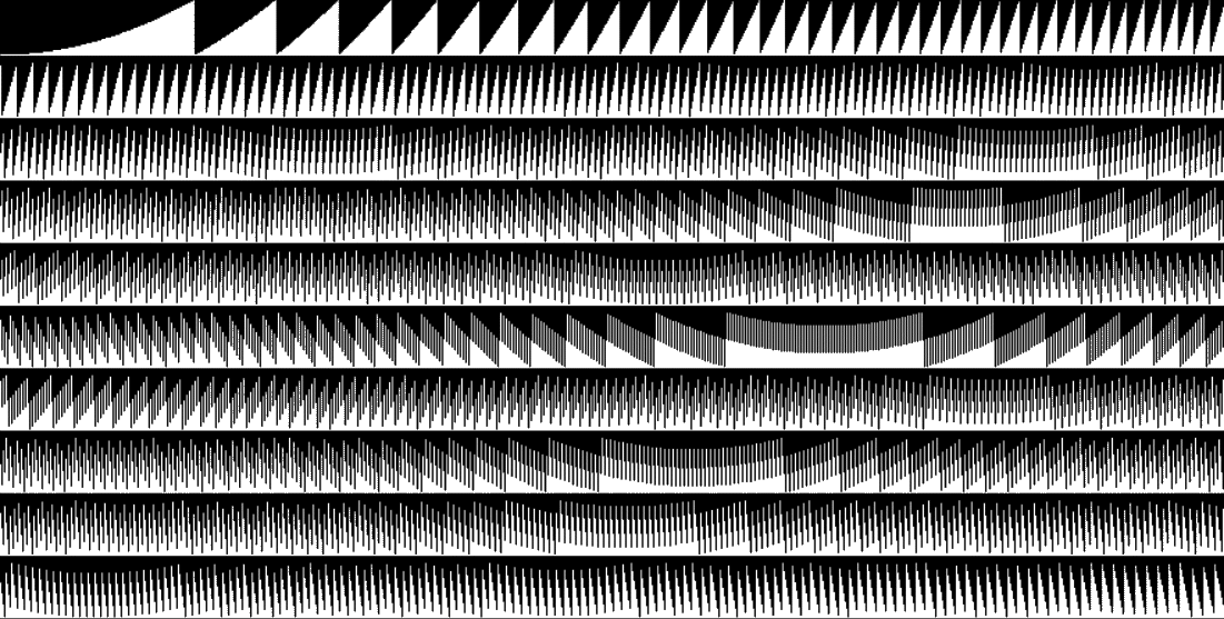
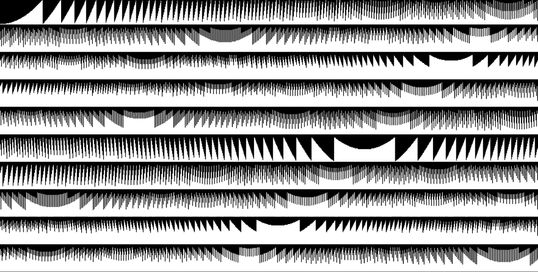
The final two digits form palindromes too. And this time we don’t get just triangles, but curves too. But that’s in base 10. What happens with the trailing triangular digits in other bases? Well, here’s the final triangular digit creating more altars of mathness in different bases (note that the altars are more elaborate in even bases):
Final triangular digit in base 4
Final triangular digit in b5
Final triangular digit in b6
Final triangular digit in b7
Final triangular digit in b8
Final triangular digit in b9
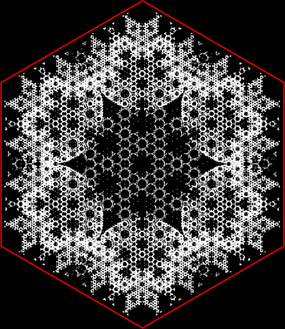
Final triangular digit in b14
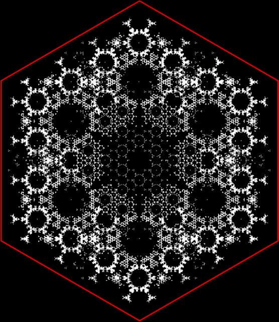
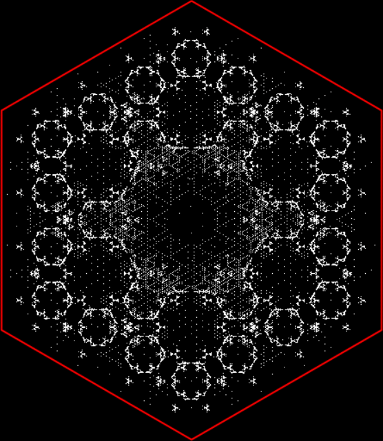
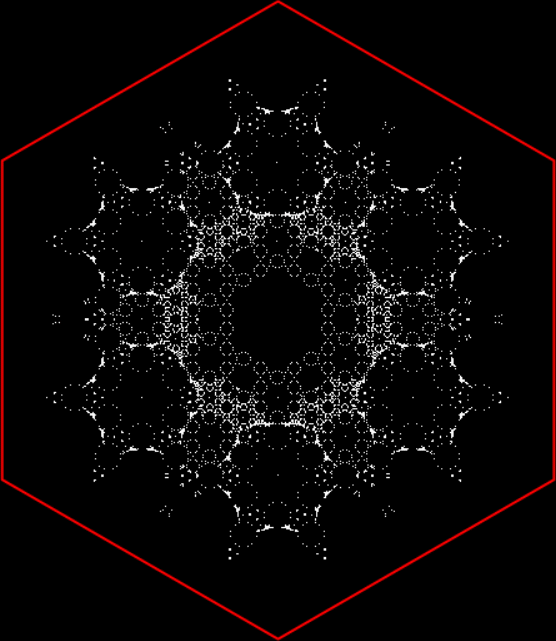
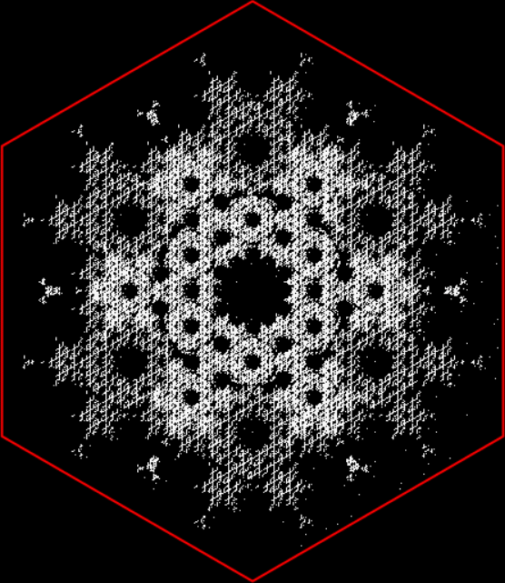
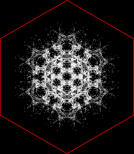
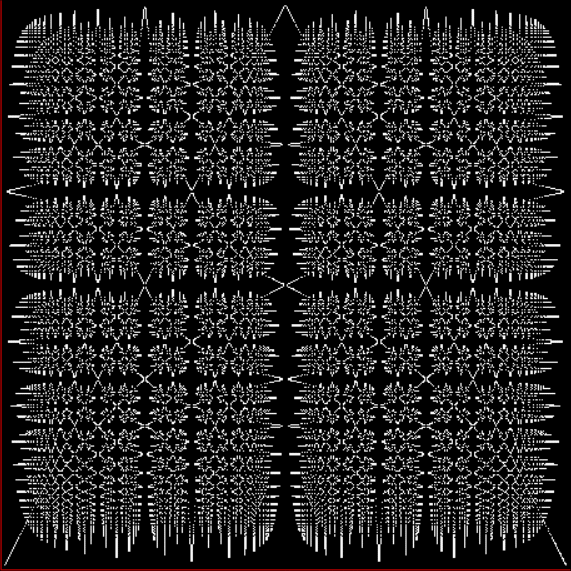
And here’s the graph for the final triangular digit in base 100:
Final triangular digit in b100
The graph for final single digit in b100 should look familiar, because it’s identical to the graph for final double triangular digits in b10:
Final two digits of triangulars in b10
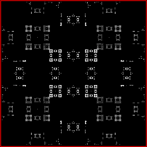
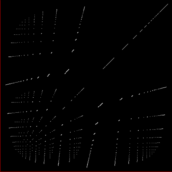
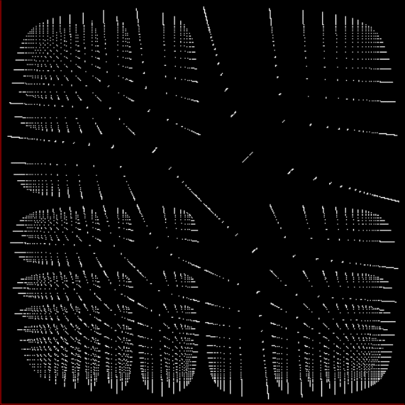
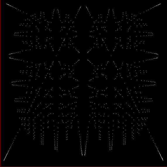
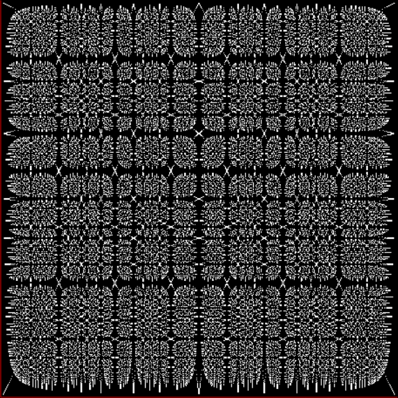
That’s because two digits in b10 are equivalent in one digit in b100, four digits in b10 are equivalent to two digits in b100, and so on. But b100 can’t capture three digits in b10 (the graph is again adjusted so that 999 fits into the same space as 9 and 99 above):
Final three triangular digits in b10
If you compress the x-axis for that graph, you can see how long the symmetries are:
Final three triangular digits in b10 (x-axis / 2)
Final three triangular digits in b10 (x-axis / 4)
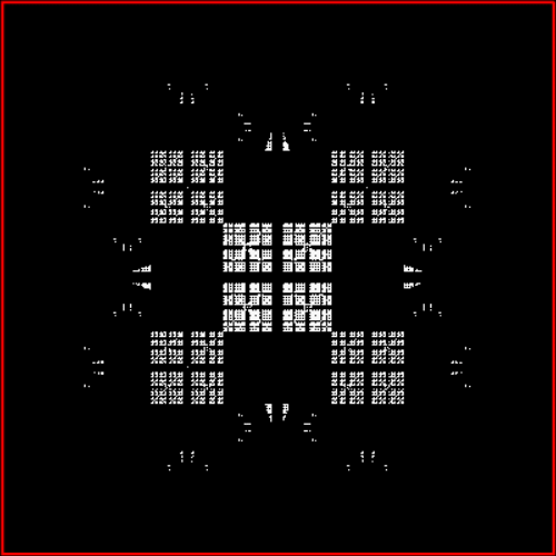
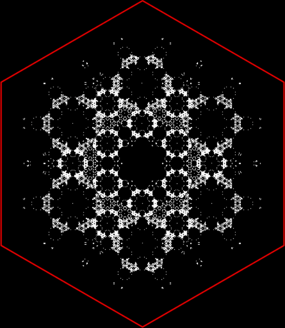
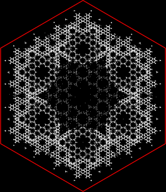
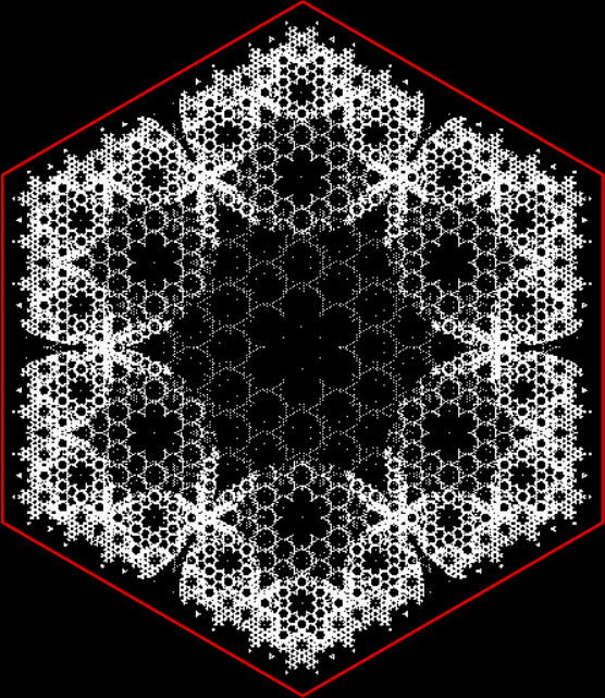
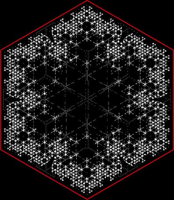
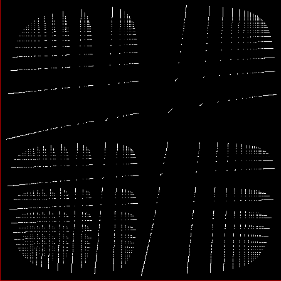
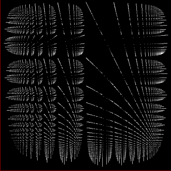
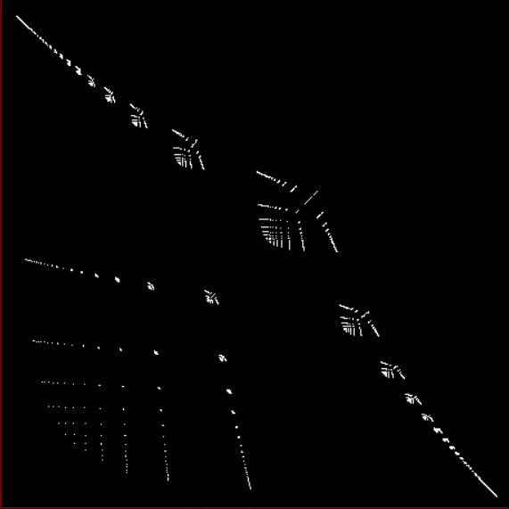
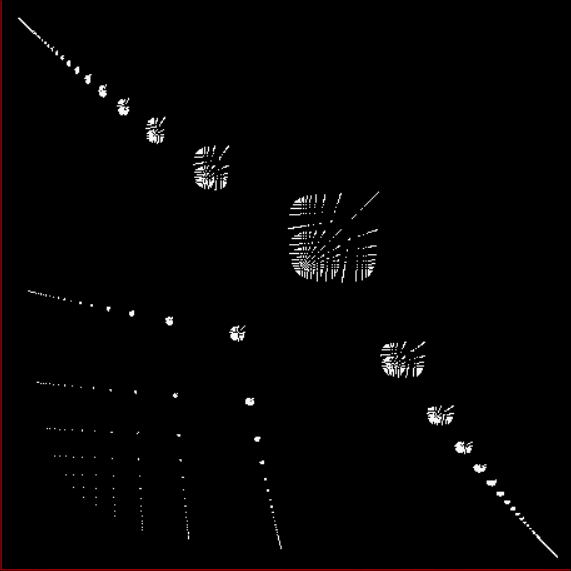
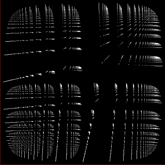
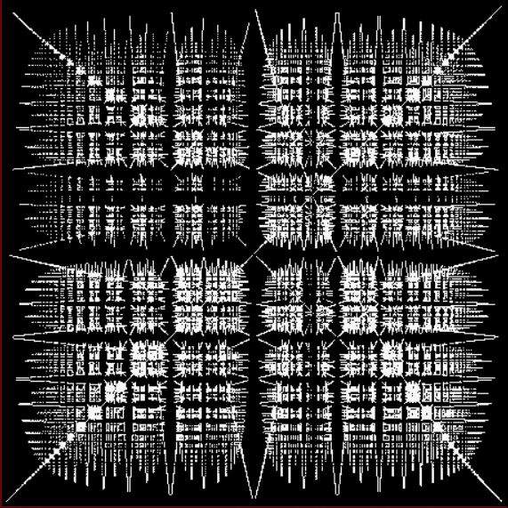
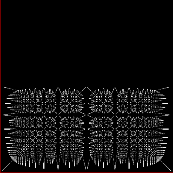
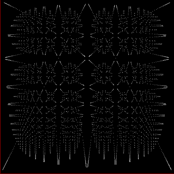
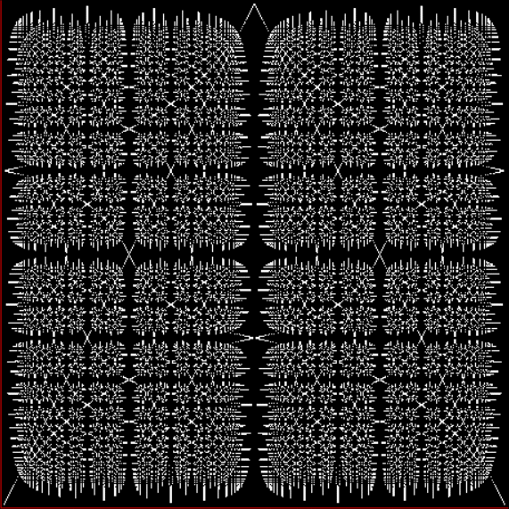
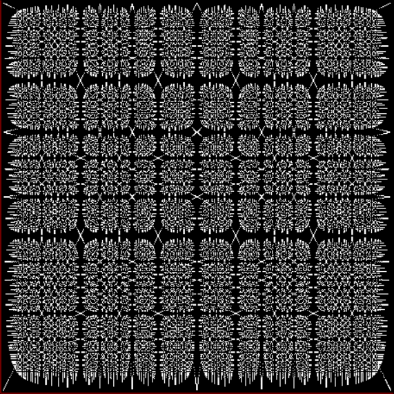
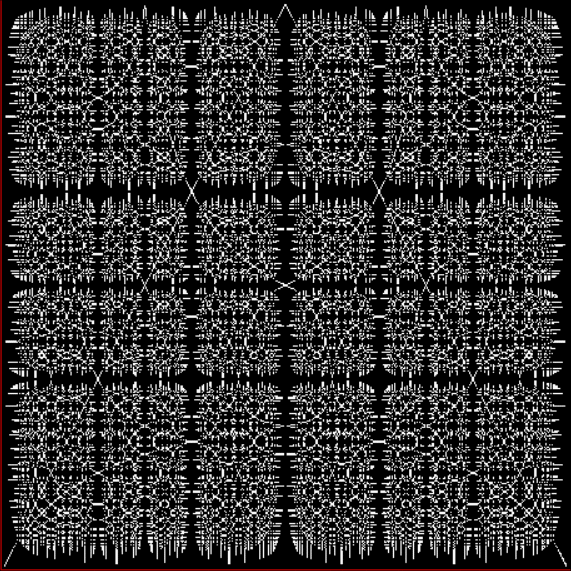
The final four digits of the triangulars in b10 create even longer symmetries:
Final quadruple triangular digits in b10
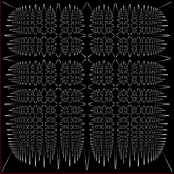
Final quadruple triangular digits in b10 (x-axis / 2)
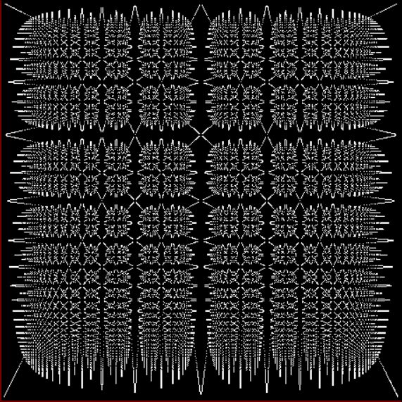
Final quadruple triangular digits in b10 (x-axis / 8)
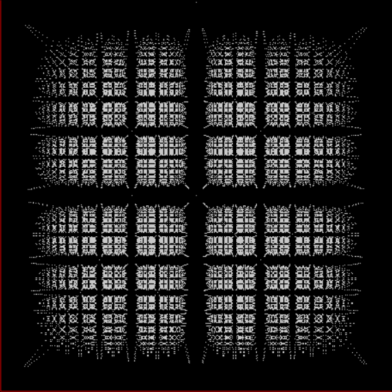
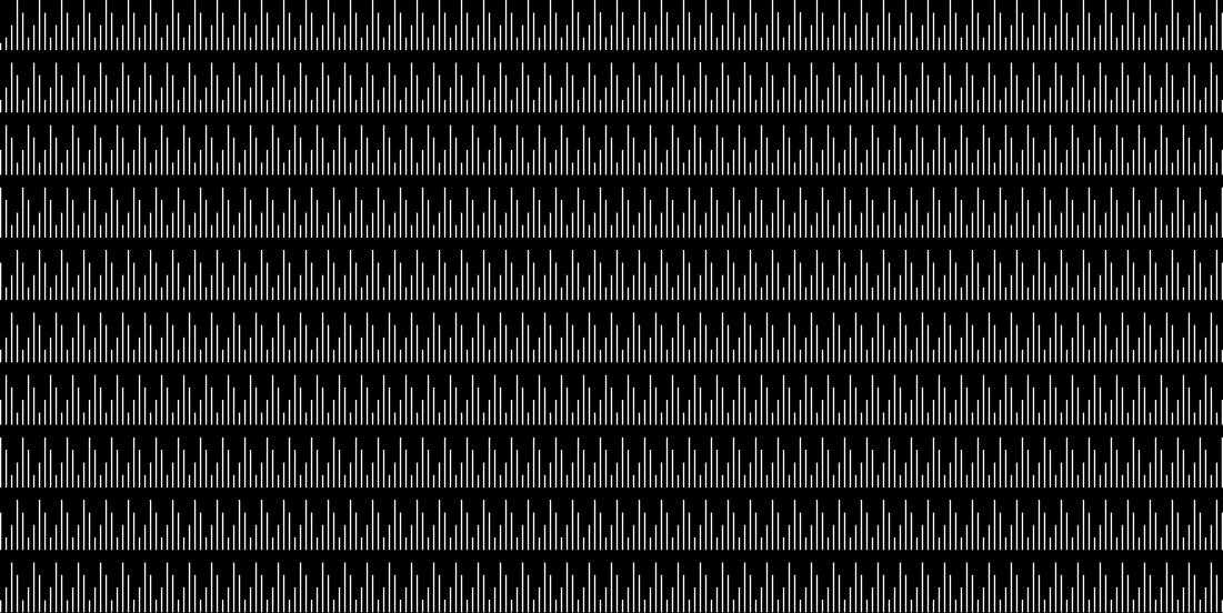
Note how, as the length of the final digits rises, you need to compress the x-axis more and more to see the symmetries. But integer sequences obviously don’t end with the counting numbers and triangulars. What about squares and powers of n? What about primes and Fibonacci numbers? Here’s the final two digits of the squares — 1, 4, 9, 16, 25, 49, 64, 81, 100, 121, 144, 169… — in b10:
Final two digits of the squares in b10
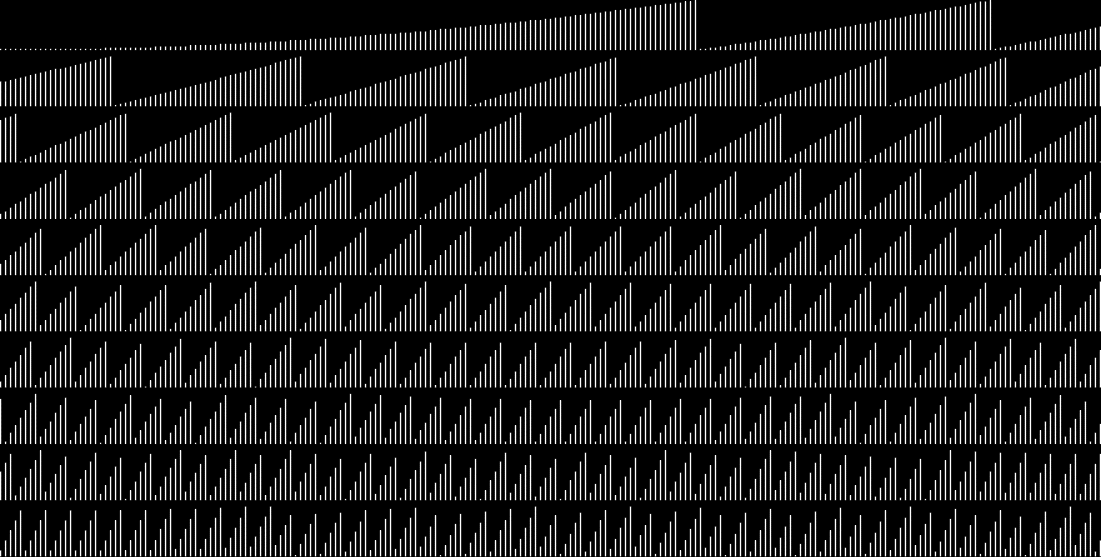
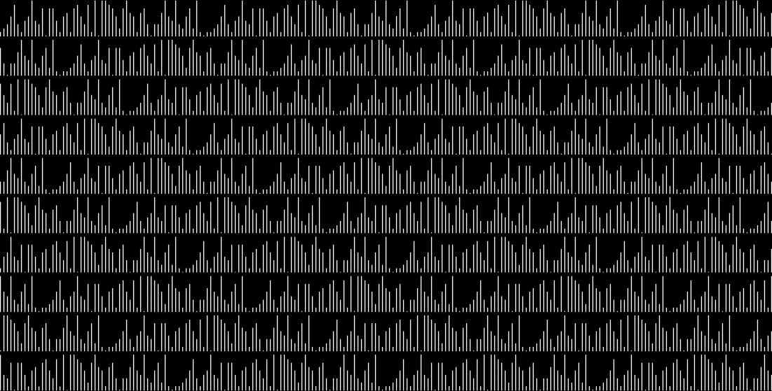
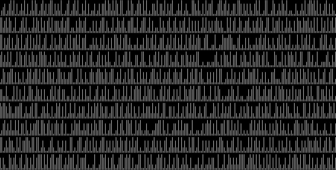
It’s reminiscent of the triangular numbers (so are the final-digit graphs for other polygonal numbers). So what about the powers of 2? That’s 2, 4, 8, 16, 32, 64, 128, 256, 512, 1024… Here’s the graph for final single digits of 2^p in b10:
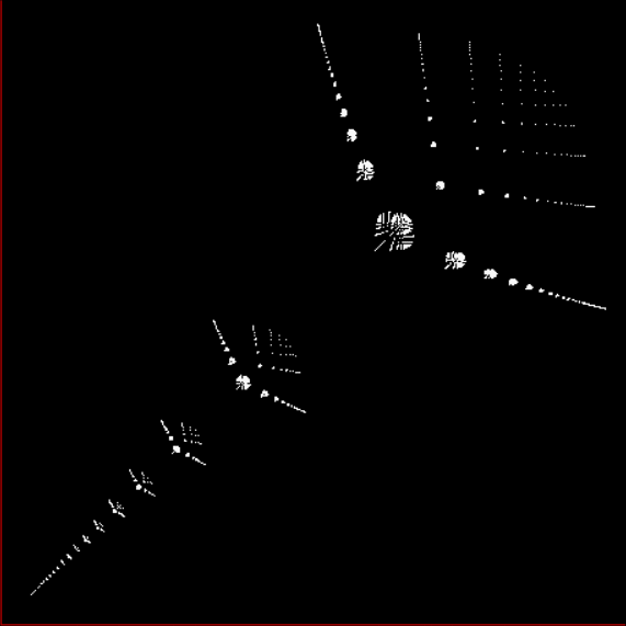
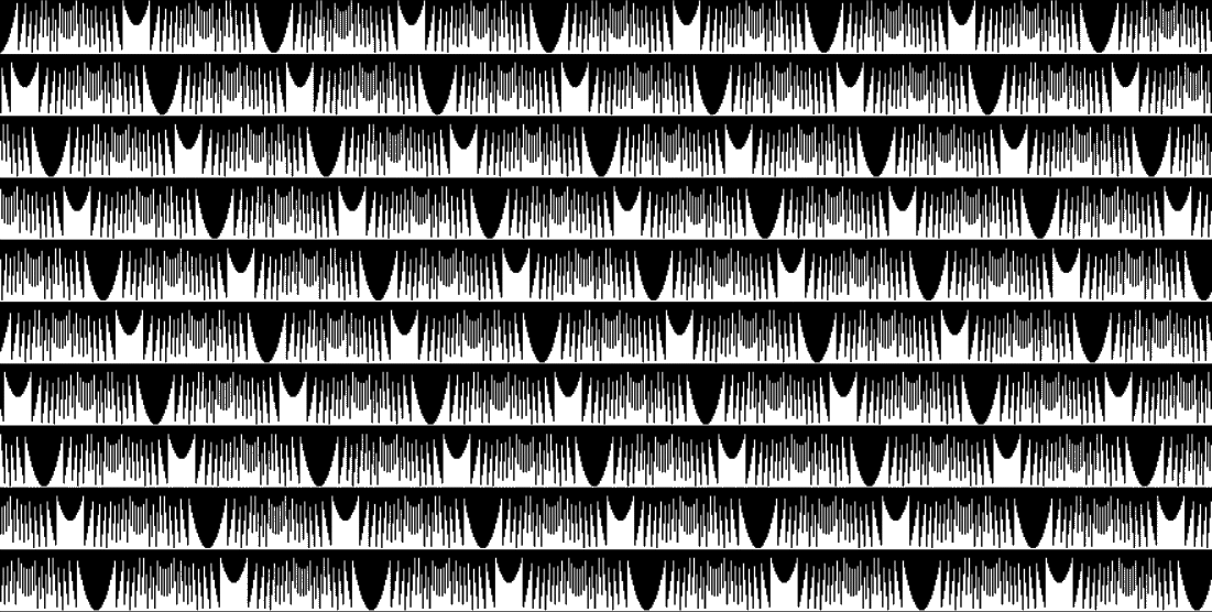
Final single digits of 2^p in b10
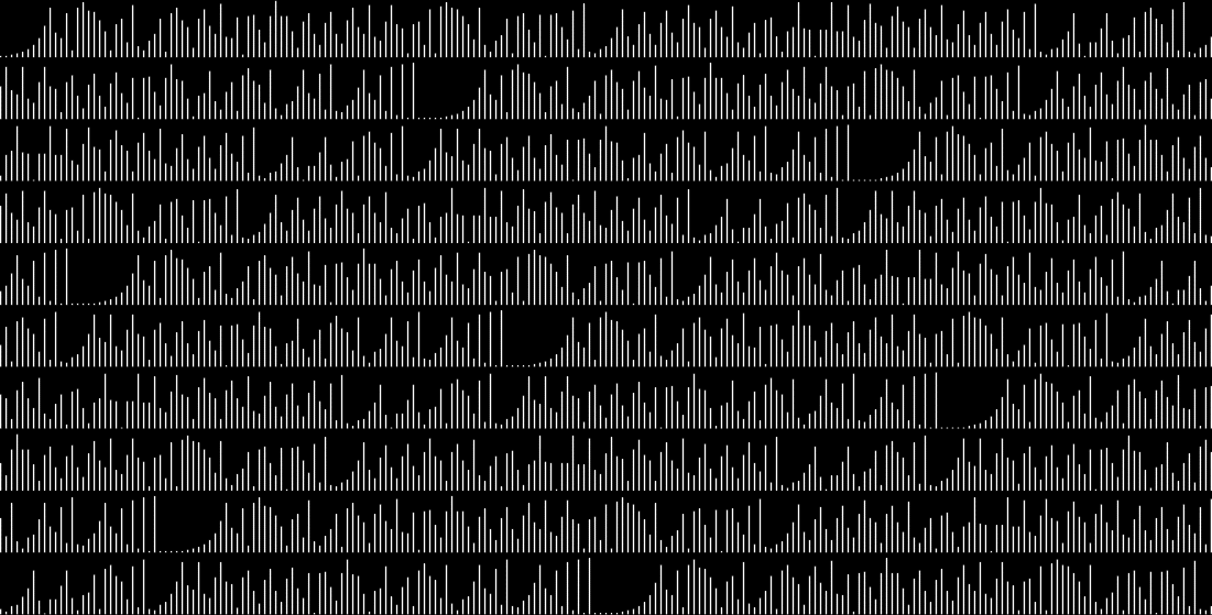
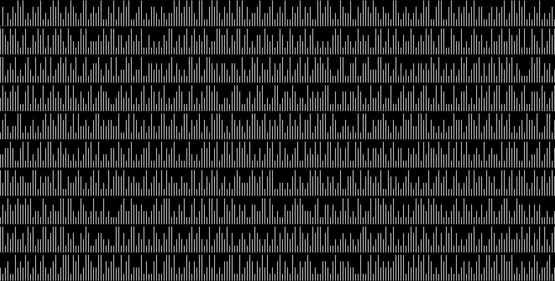
This time there’s repetition, but not symmetry. Here’s the graph for final double digits, or 2-digits, of 2^p in b10:
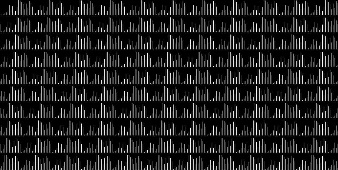
Final 2-dig of 2^p in b10
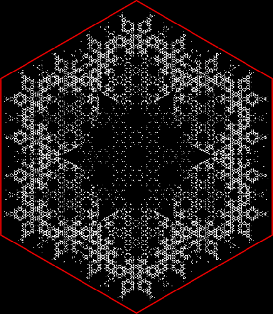
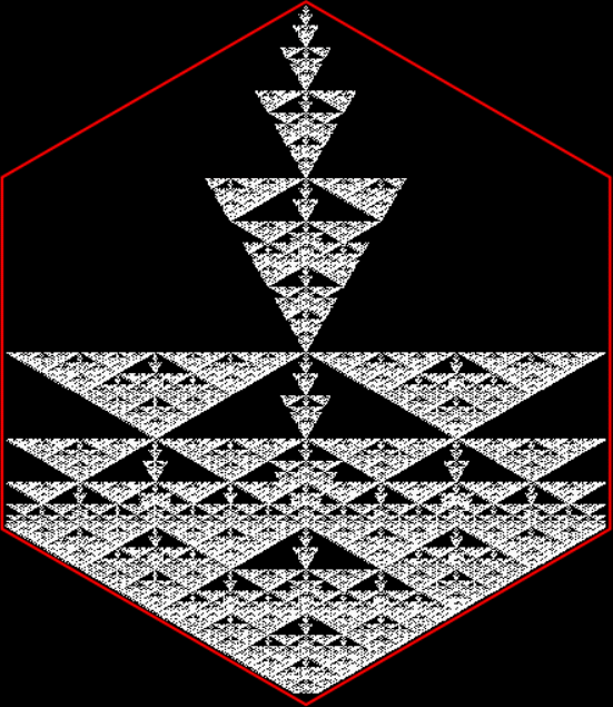
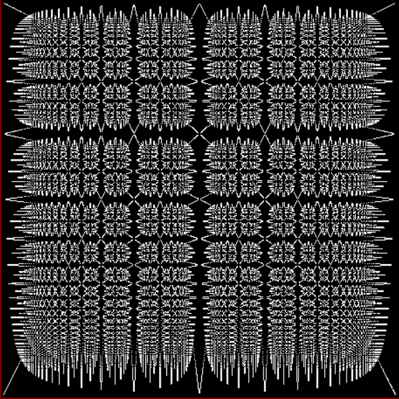
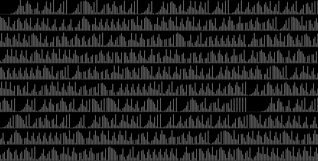
Now the graph looks a little like a range of eroded mountains. Now try dig-4, the final four digits of 2^p in b10:
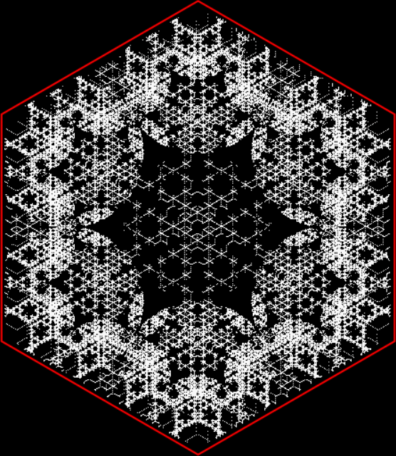
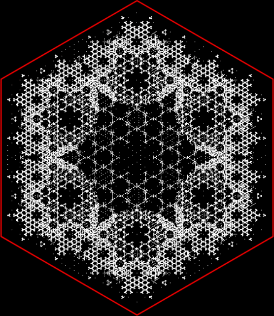
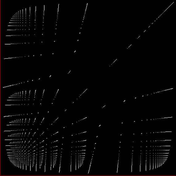
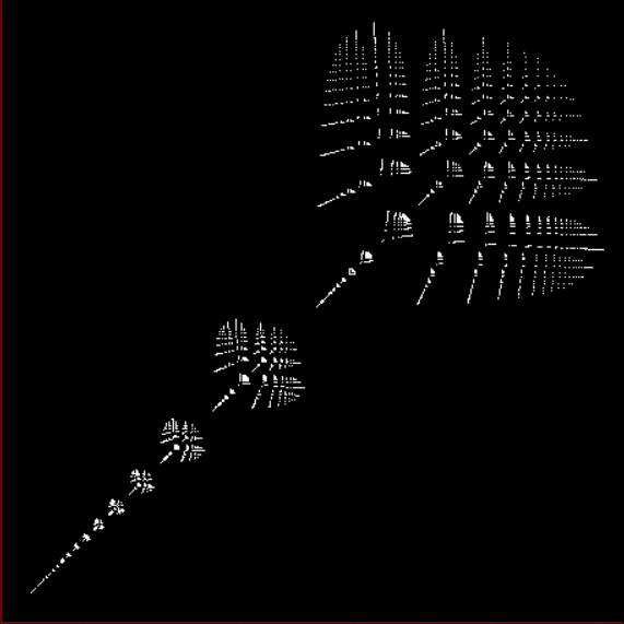
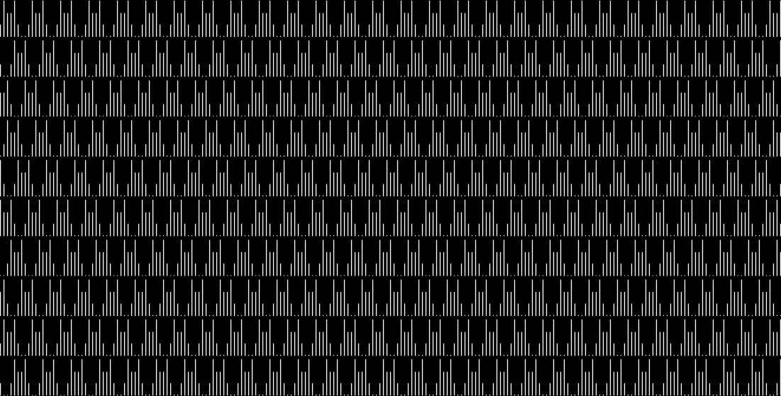
Final 4-dig of 2^p in b10
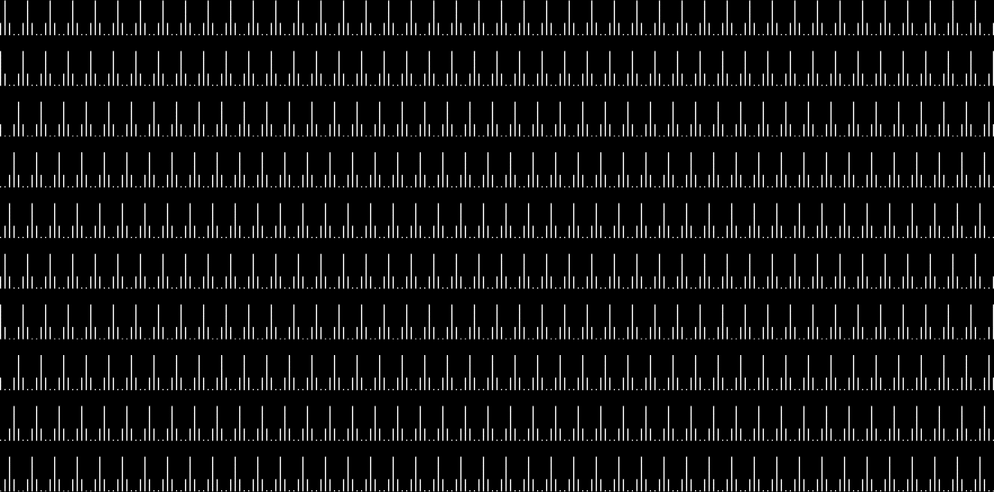
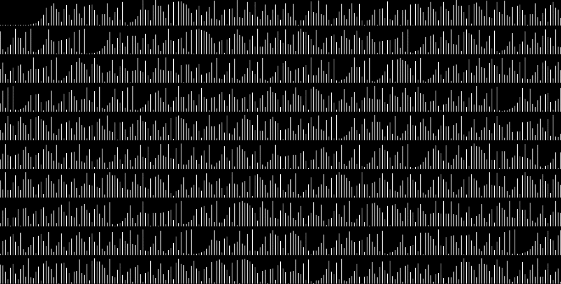
The patterns are similar to those of dig-2 and don’t need compressing in the x-axis. This similarity and lack of need for compression are true of any number of final digits in 2^p. The final 10 digits look like this:
Final 10-dig of 2^p in b10
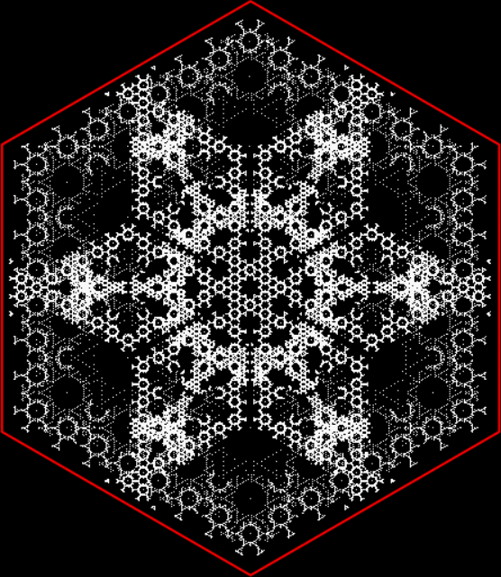
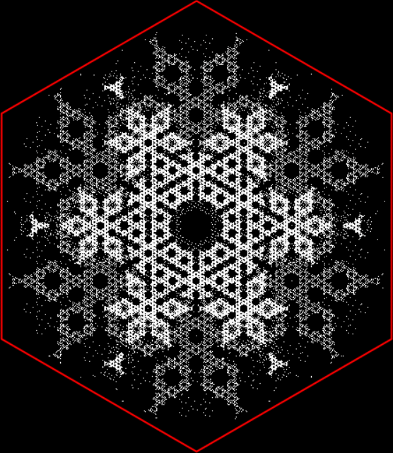
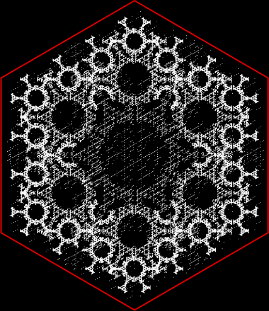
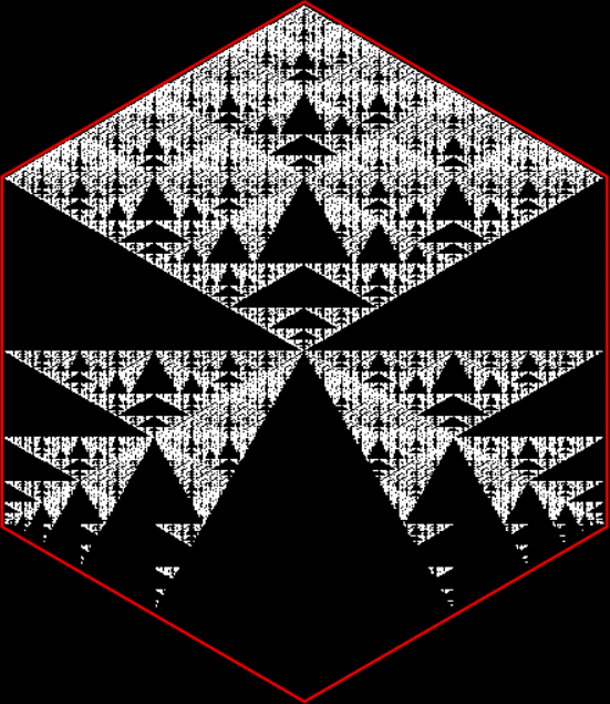
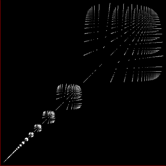
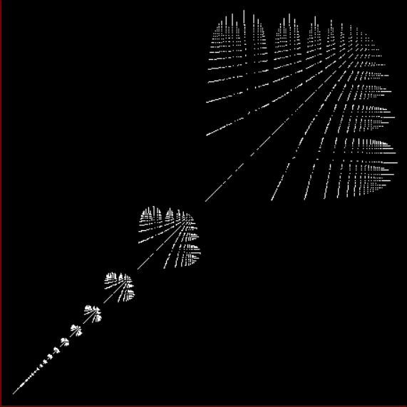
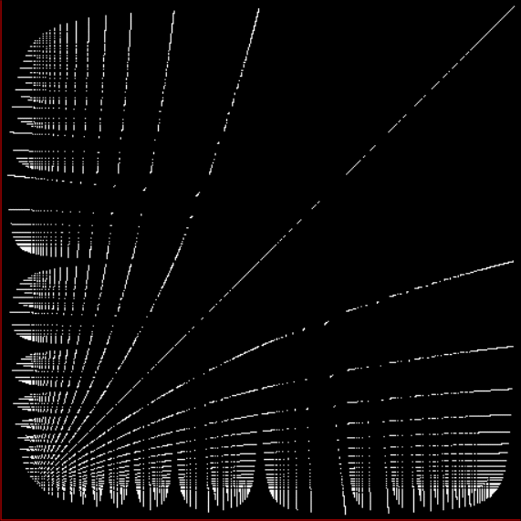
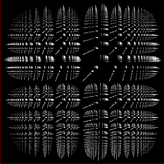
And the final 20 and 30 digits like this:
Final 20-dig of 2^p in b10
Final 30-dig of 2^p in b10
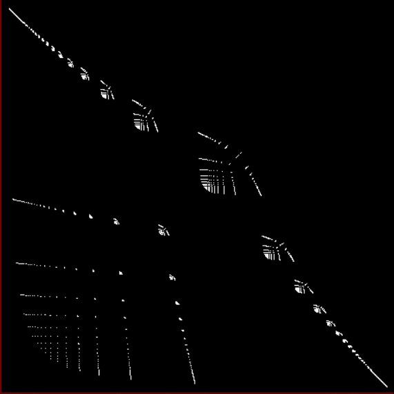
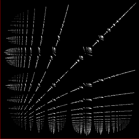
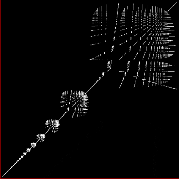
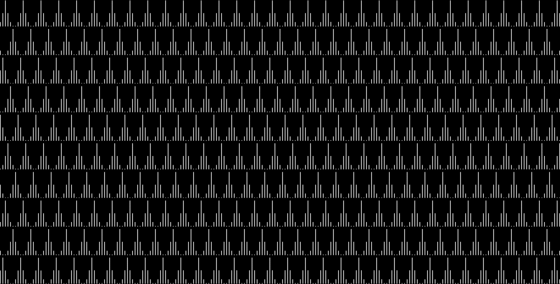
Powers don’t behave like polygonals: the finals are fractals. That is, the final digits create similar patterns at all scales: 1-dig, 2-dig, 10-dig, 100-dig, 1000-dig and so on. That’s true in other bases:
Final 5-dig of 3^p in b2
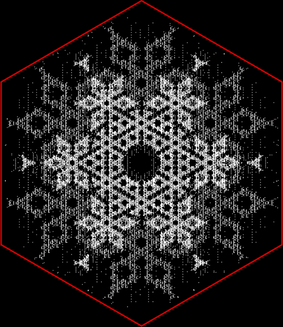
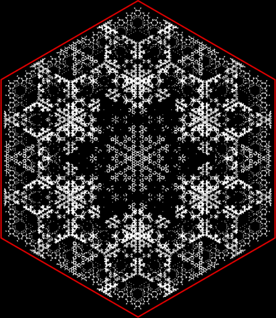
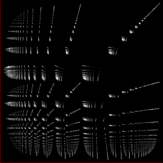
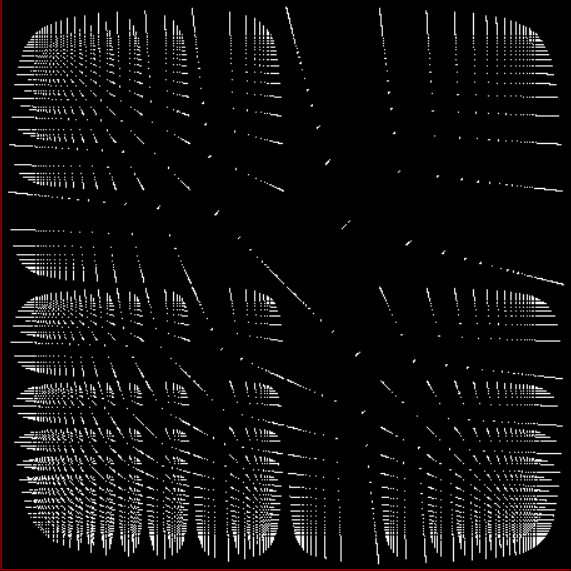
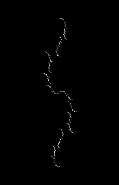
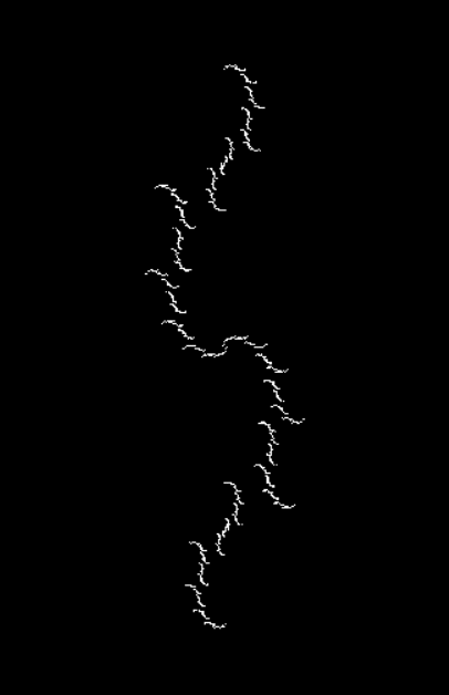
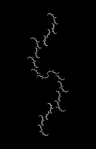
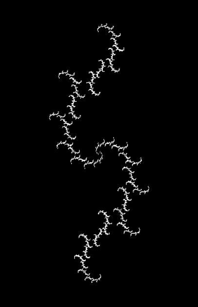
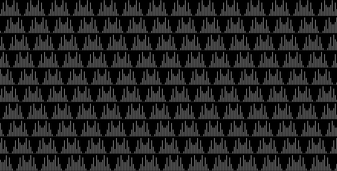
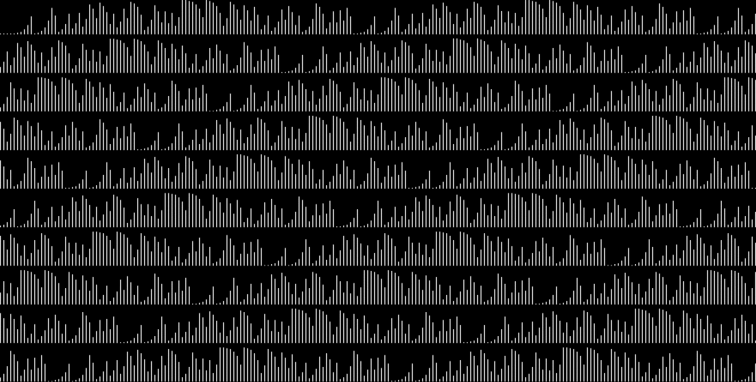
But a glimpse of b2 is all you’re going to get of other bases. There are other fish to fry — Fibonacci fish. The Fibonacci sequence, whose terms are equal to the sum of the previous two numbers (after seeding with “1, 1”), starts like this: 1, 1, 2, 3, 5, 8, 13, 21, 34, 55, 89, 144, 233, 377, 610, 987, 1597, 2584, 4181, 6765, 10946, 17711, 28657, 46368, 75025, 121393, 196418, 317811… And what about the graphs for final fib-digits? As you’ll see, final Fib-digits are fractal too. Indeed, Fibonacci final-graphs look like 2-power final-graphs (in a way, Fibonacci numbers are powers of φ = 1.6180339887498948482…). The patterns are similar at all scales. And they remind me of the skyline of a ruined city in an Oriental tale, with collapsed domes and crumbling minarets:
Final 1-dig of Fibonacci numbers in b10
Final 2-fibdig in b10
Final 3-fibdig in b10
Final 4-fibdig in b10

Final 5-fibdig in b10
Final 10-fibdig in b10
Final 15-fibdig in b10
Final 20-fibdig in b10
Final 25-fibdig in b10
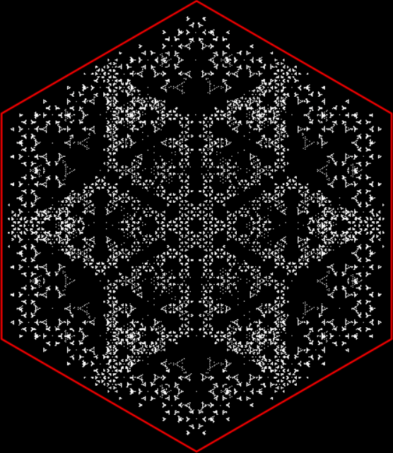
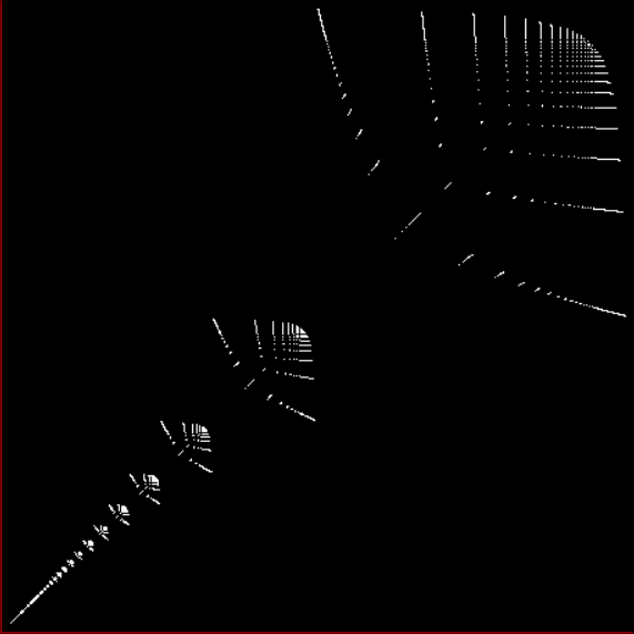
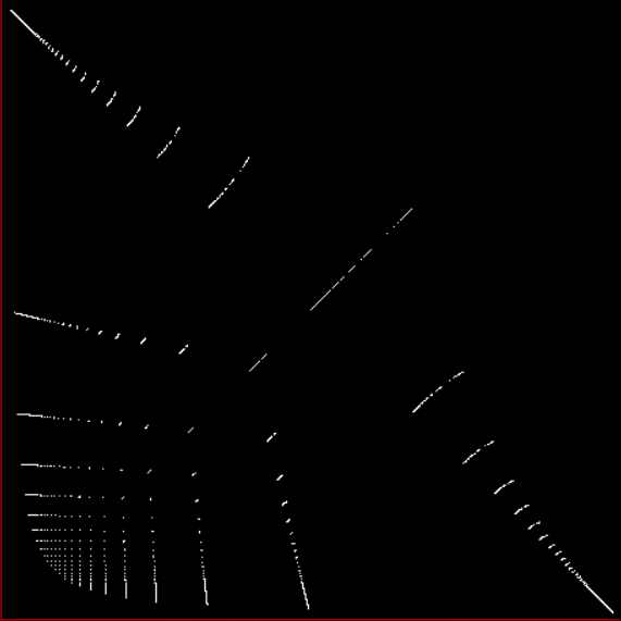
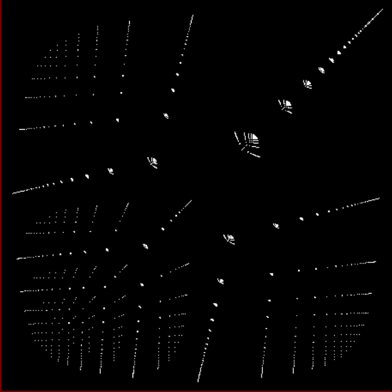
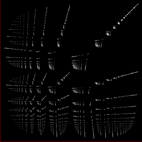
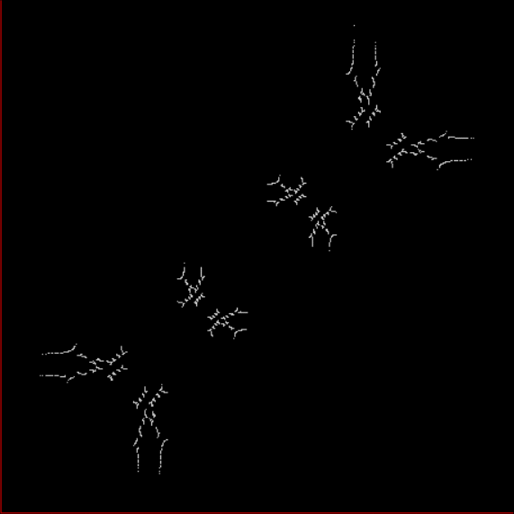
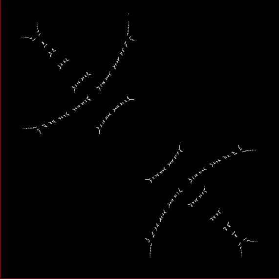
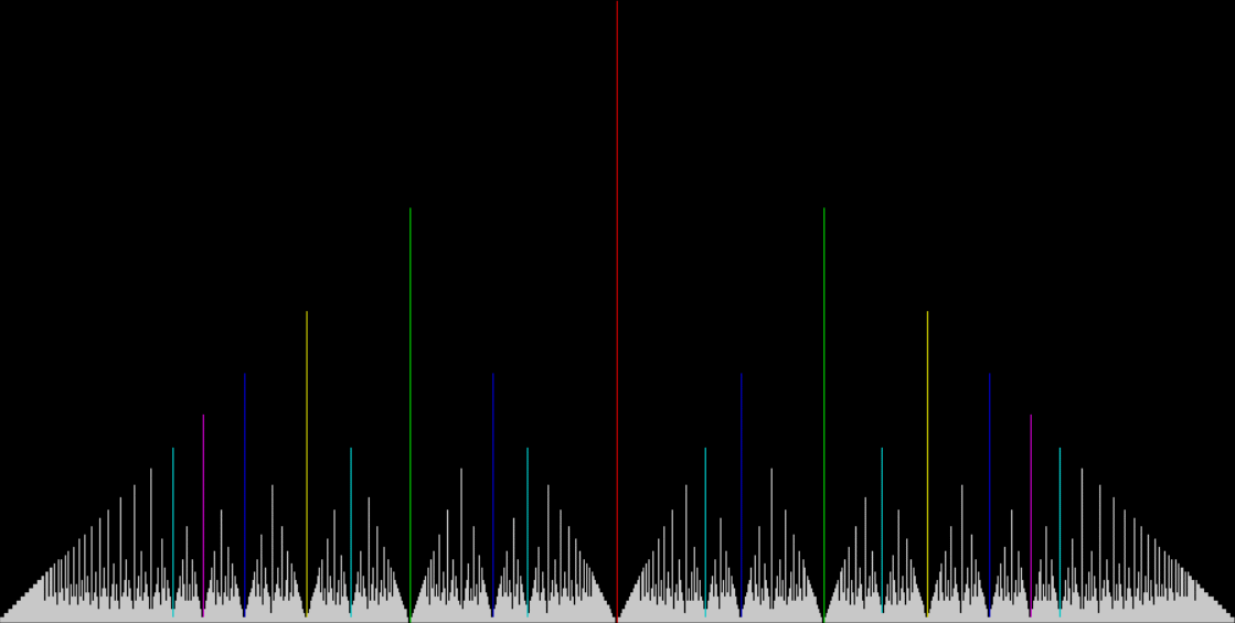
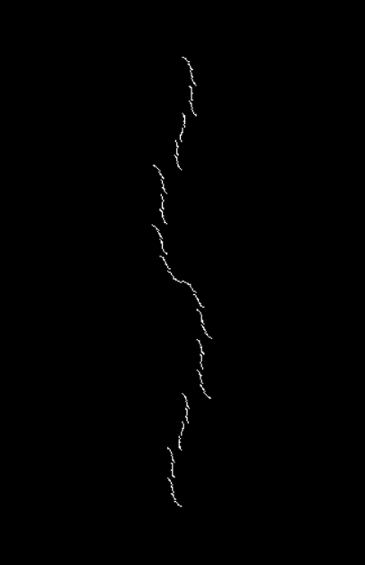
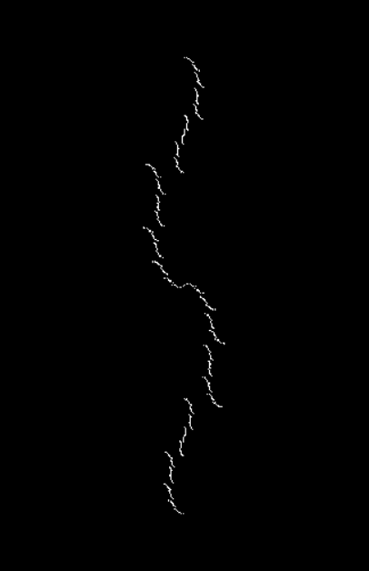
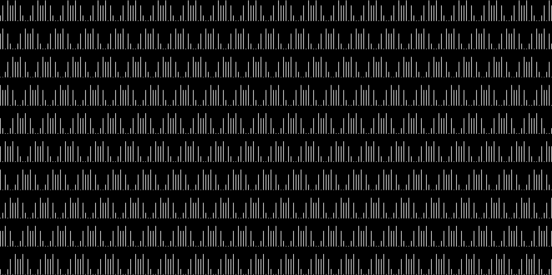
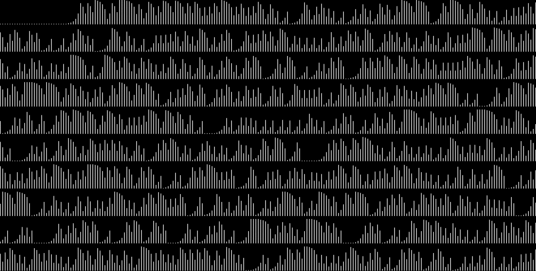
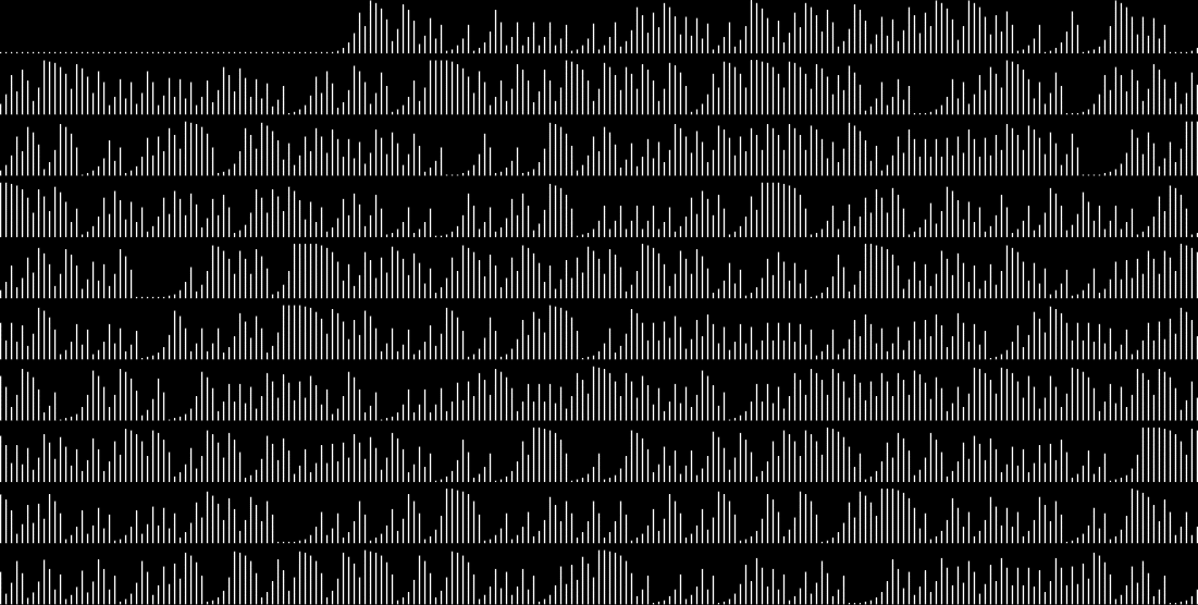
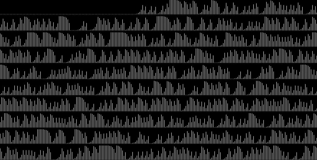
So final fibdigs are fractal. But final prime digits aren’t:
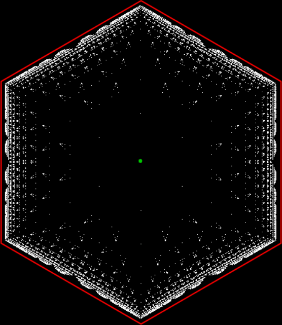
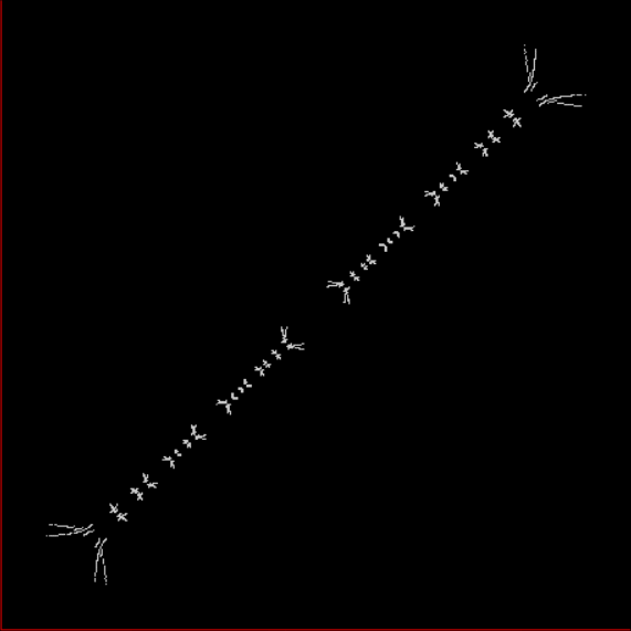
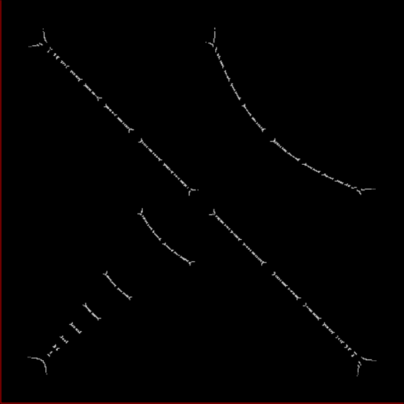
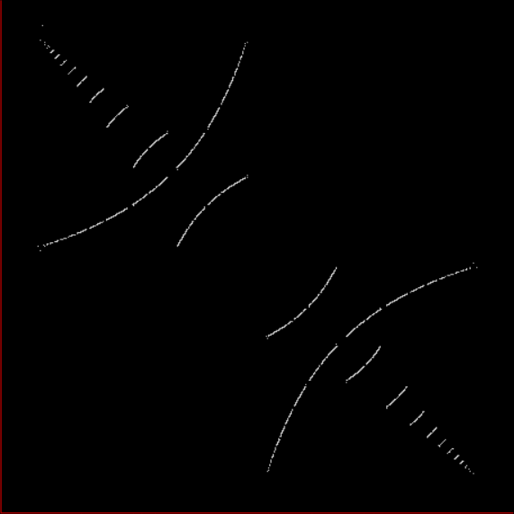
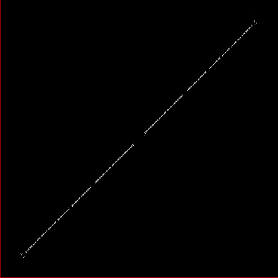
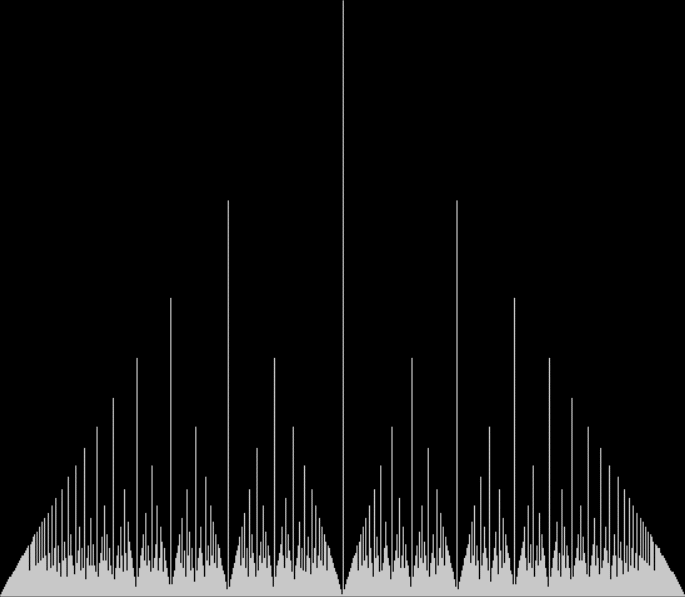
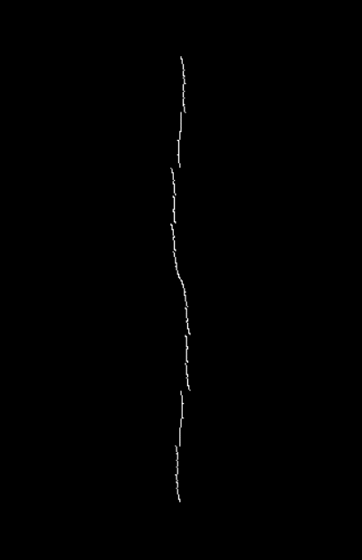
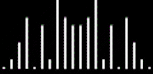
Final 1-digit of primes in b10
Final 1-digit of primes in b5
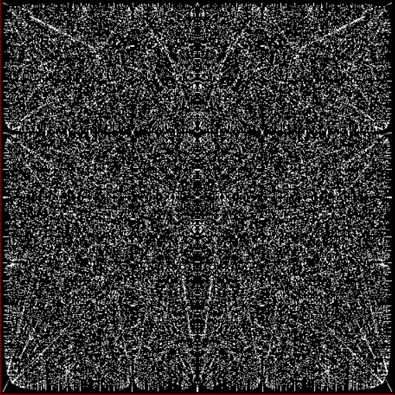
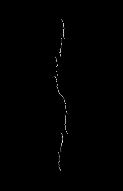
Final 2-digit of primes in b10
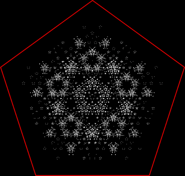
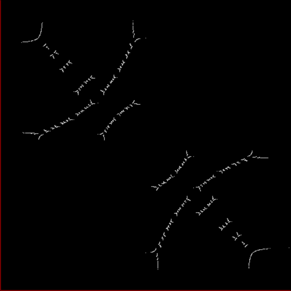
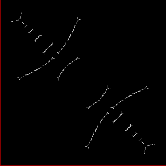
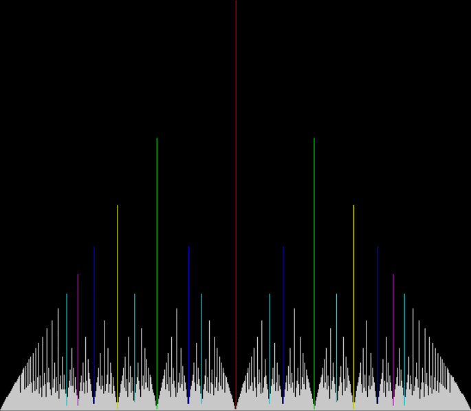
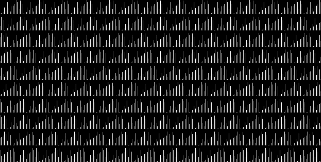
Primes aren’t final-digitally fractal like Fibonaccis and powers of 2. But there’s occasional symmetry in the prime fin-digs. I’ve marked some palindromic patterns in red and green:
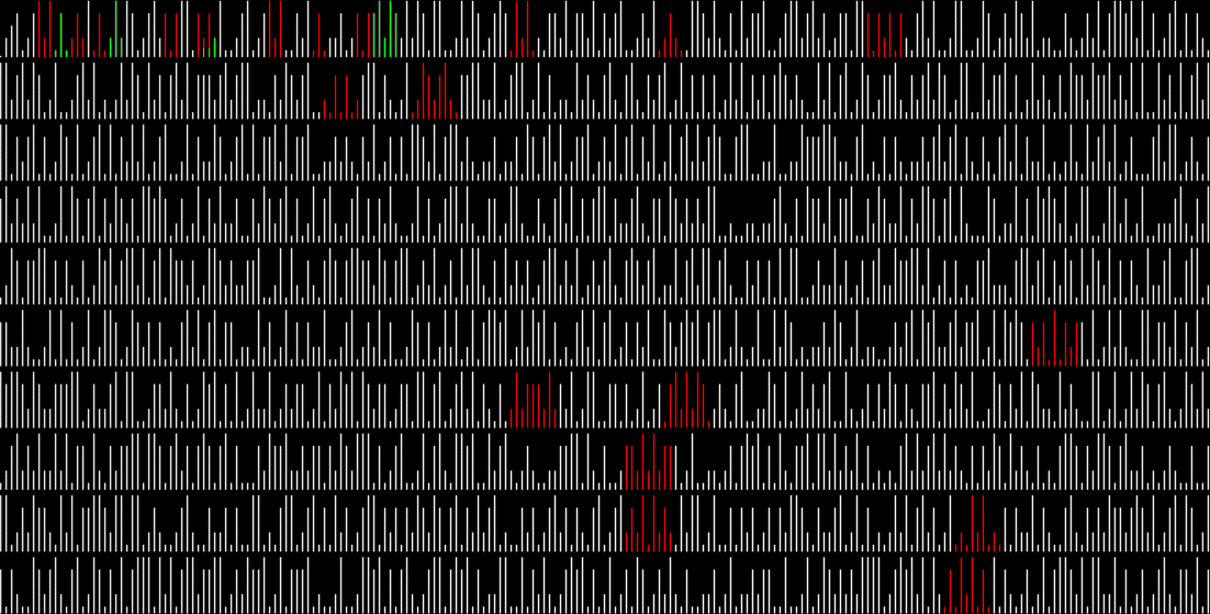
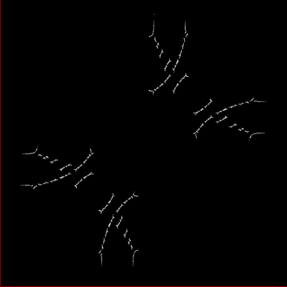
Palindromic patterns in final 1-digits of the primes in b10 (click for larger)
The palindromic patterns, or pal-pats, in the primes look like the altars of mathness in the triangulars. They’re created by digital palindromes like these:
19, 23, 29 (c=3)
347, 349, 353, 359, 367 (c=5)
937, 941, 947, 953, 967, 971, 977 (c=7)
1951, 1973, 1979, 1987, 1993, 1997, 1999, 2003, 2011 (c=9)
26423, 26431, 26437, 26449, 26459, 26479, 26489, 26497, 26501, 26513 (c=10)
Here are the first few pal-pats in the primes (note that 157, 163, 167 and 163, 167, 173 overlap):
2, 3, 5, 7, 11, 13, 17, 19, 23, 29, 31, 37, 41, 43, 47, 53, 59, 61, 67, 71, 73, 79, 83, 89, 97, 101, 103, 107, 109, 113, 127, 131, 137, 139, 149, 151, 157, 163, 167, 173, 179, 181, 191, 193, 197, 199, 211, 223, 227, 229, 233, 239, 241, 251, 257, 263, 269, 271, 277, 281, 283, 293, 307, 311, 313, 317, 331, 337, 347, 349, 353, 359, 367, 373, 379, 383, 389, 397, 401, 409, 419, 421, 431, 433, 439, 443, 449, 457, 461, 463, 467, 479, 487, 491, 499, 503, 509, 521, 523, 541, 547, 557, 563, 569, 571, 577, 587, 593, 599, 601, 607…
And are there palindromes among the final 2-digits, 3-digits and higher n-digits of the primes in different bases? Yes, you can easily find some. But I haven’t put them on a graph yet:
Base 10 (2-dig)
58789, 58831, 58889 (c=3)
286873, 286927, 286973 (c=3)
360649, 360653, 360749 (c=3)
404851, 404941, 404951 (c=3)
590437, 590489, 590537 (c=3)
623071, 623107, 623171 (c=3)
651517, 651587, 651617 (c=3)
Base 6 (2-dig)
300335, 300401, 300441, 300501, 300535 (c=5) (23459 to 23531 in base 10)
1030255, 1030331, 1030351, 1030431, 1030455 (c=5) (50651 to 50723 in b10)
1140451, 1140501, 1140521, 1141001, 1141051 (c=5) (59791 to 59863 in b10)
1402451, 1402545, 1403031, 1403045, 1403051 (c=5) (78367 to 78439 in b10)
1435431, 1435451, 1435505, 1435551, 1440031 (c=5) (82891 to 82963)
2400505, 2401001, 2401015, 2401101, 2401105 (c=5) (124601 to 124673)
2442235, 2442311, 2442351, 2442411, 2442435 (c=5) (130127 to 130199)
2444215, 2444225, 2444311, 2444325, 2444415 (c=5) (130547 to 130619)
2533105, 2533121, 2533215, 2533221, 2533305 (c=5) (136769 to 136841)
Base 4 (3-dig)
20013013, 20013133, 20020013 (c=3) (33223 to 33287 in base 10)
21031111, 21031303, 21032111 (c=3) (37717 to 37781)
22310011, 22310333, 22311011 (c=3) (44293 to 44357)
33030121, 33031001, 33031121 (c=3) (62233 to 62297)
102031333, 102032131, 102032333 (c=3) (74623 to 74687)
110013121, 110013311, 110020121 (c=3) (82393 to 82457)
Base 3 (3-dig)
112121020012, 112121021211, 112121022021, 112121100211, 112121101012 (c=5) (287393 to 287501 in base 10)
202002212002, 202002212101, 202002220001, 202002221101, 202010000002 (c=5) (395741 to 395849)
1001012111212, 1001012112202, 1001012121022, 1001012121202, 1001012122212 (c=5) (555143 to 555251)
1010112112012, 1010112112201, 1010112120222, 1010112121201, 1010112200012 (c=5) (601079 to 601187)
1011202211211, 1011202212212, 1011202220022, 1011202221212, 1011202222211 (c=5) (625369 to 625477)
Base 2 (5-dig)
101110001111101, 101110010000111, 101110010001001, 101110010100111, 101110010111101 (c=5) (23677 to 23741 in base 10)
10000001000111101, 10000001001011001, 10000001001110001, 10000001001111001, 10000001001111101 (c=5) (66109 to 66173)
10111100110011011, 10111100110011111, 10111100110111001, 10111100110111111, 10111100111011011 (c=5) (96667 to 96731)
11010000111110001, 11010001000001101, 11010001000011001, 11010001000101101, 11010001000110001 (c=5) (106993 to 107057)
And I conjecture that you’ll get palindromes for any number of final digits in all bases. And can these palindromes be of arbitrary length? Again, I conjecture so. There are infinitely many primes and very rare patterns can occur infinitely often in an infinite set of numbers.
Post-Performative Post-Scriptum
Here’s Dan Seagrave’s classic cover for Morbid Angel’s Altars of Madness (1989):

• Morbid Angel — official website
• Dan Seagrave — official website
Elsewhere Other-Accessible…
• Formulas Focal to the Flesh — a pre-previous post paronomasizing the title of a Morbid-Angel album…