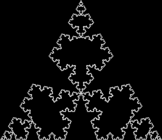
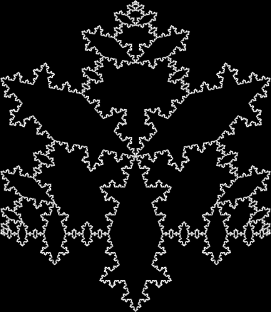
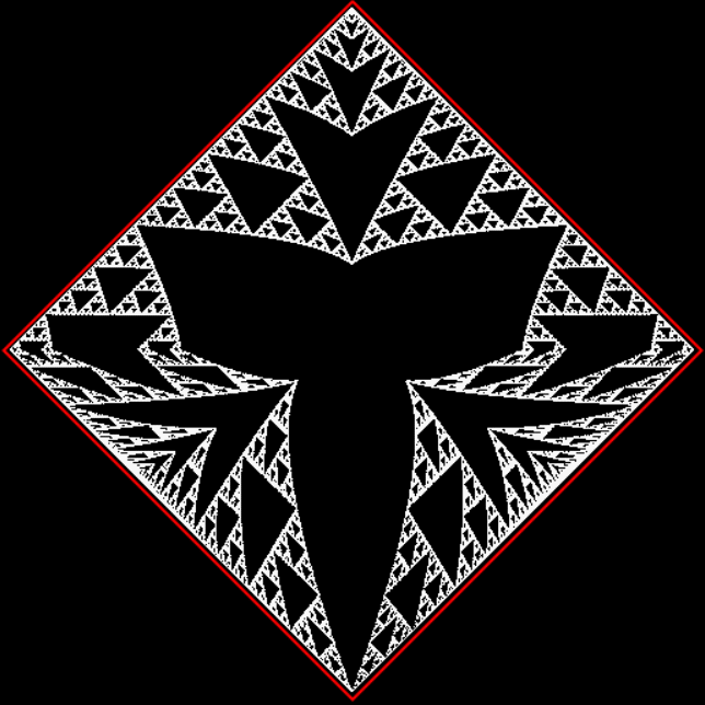
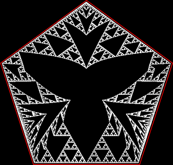
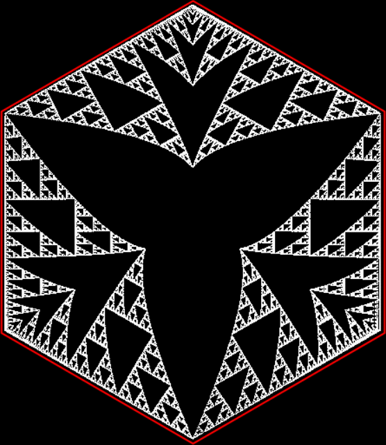
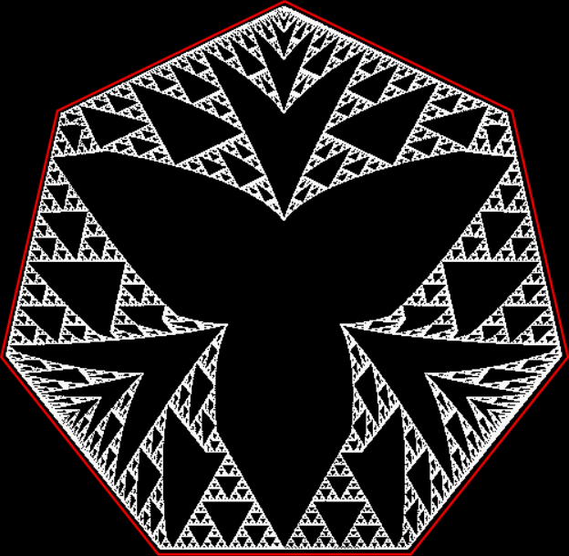
Takes on Flakes

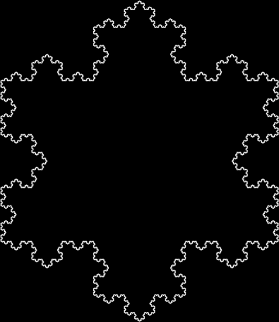
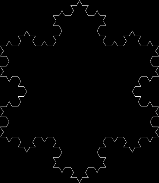
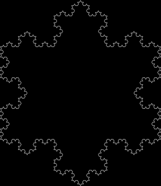
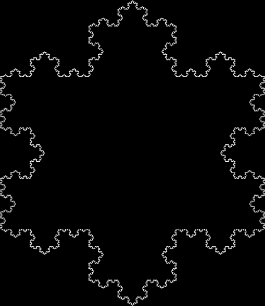
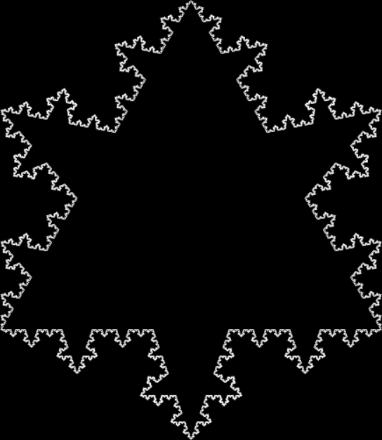
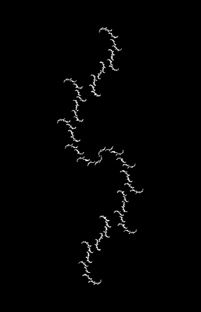
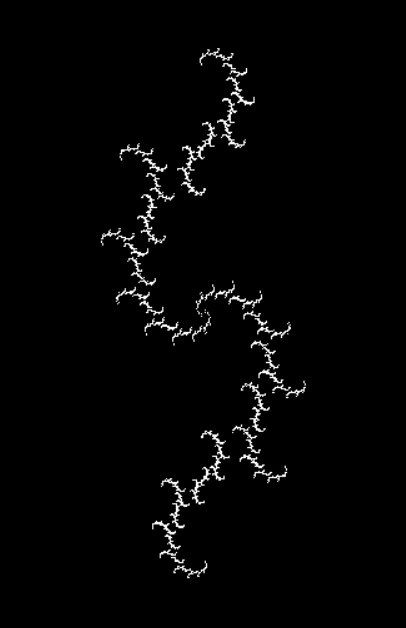
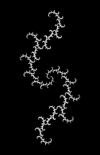
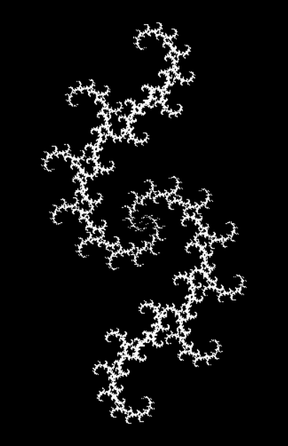
The Koch Snowflake is a fractal named after the Swedish mathematician Helge von Koch (1870-1924). It’s simple to make, attractive to see:

A Koch snowflake


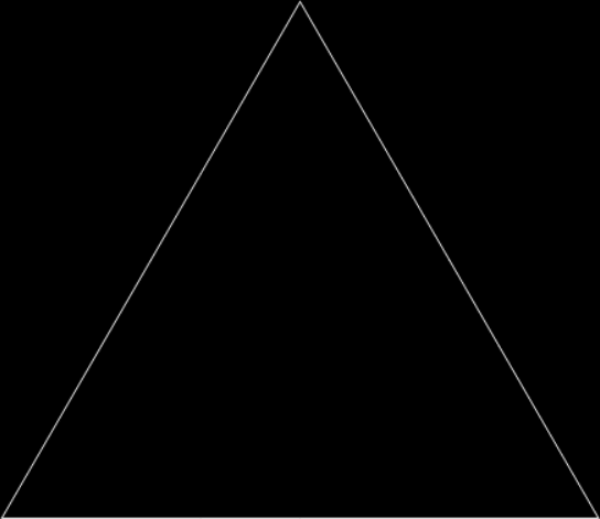
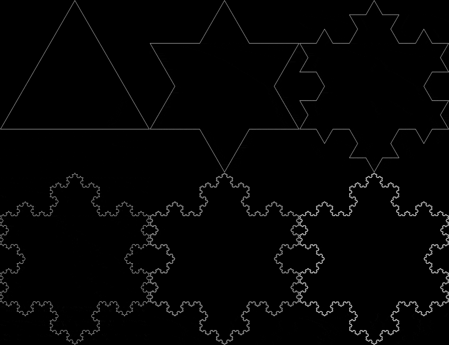
And here’s how you making it, starting with an equilateral triangle:

Make the Flake #0


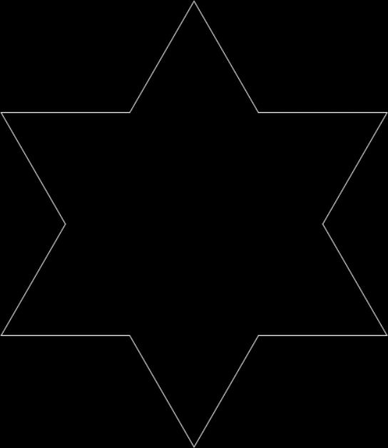
Make the Flake #1: Erect a 1/9-sized equilateral triangle on middle of each side


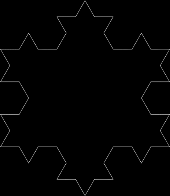
Make the Flake #2: Then a 1/81-sized equilateral triangle on the middle of each straight line created by #1


Make the Flake #3: And so on.


Make the Flake #4


Make the Flake #5


Make the Flake #6


Make the Flake #0-6 (animated at ezGif)


In the end, the Koch snowflake has an infinitely long perimeter around a finite area (see discussion at Wikipedia). The Koch anti-snowflake or un-flake also combines an infinitely long perimeter and finite area:

Koch un-Flake


You make the un-flake like this:

Make the Un-Flake #0


Make the Un-Flake #1


Make the Un-Flake #2


Make the Un-Flake #3


Make the Un-Flake #4


Make the Un-Flake #5


Make the Un-Flake #6


Make the Un-Flake #0-6 (animated at ezGif)


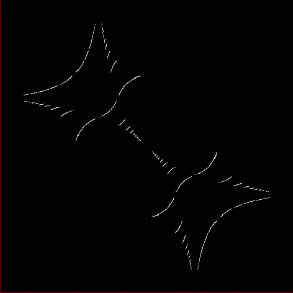
And you can combine the Koch snowflake and the Koch anti-snowflake like this:

Make the Flake+Un-Flake #0


Make the Flake+Un-Flake #1


Make the Flake+Un-Flake #2


Make the Flake+Un-Flake #3


Make the Flake+Un-Flake #4


Make the Flake+Un-Flake #5


Make the Flake+Un-Flake #6


Make the Flake+Un-Flake #0-6 (animated at ezGif)


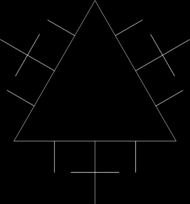
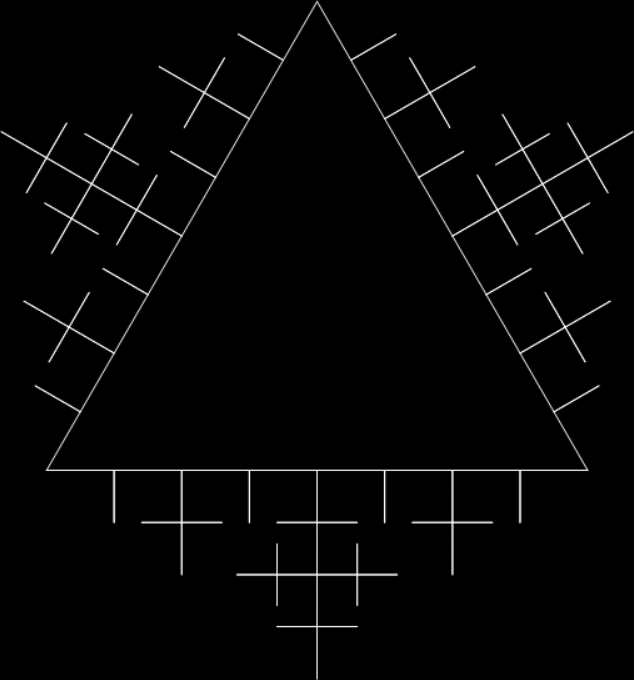
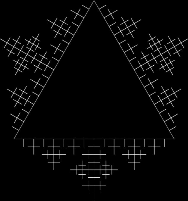
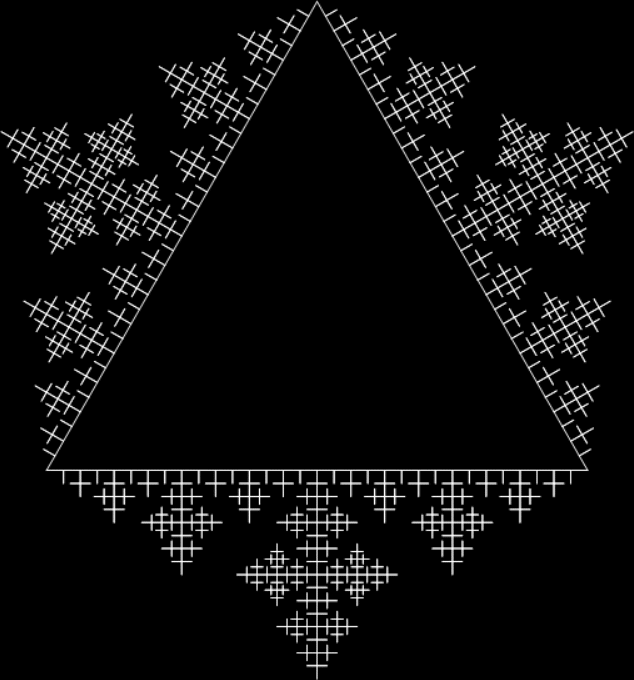
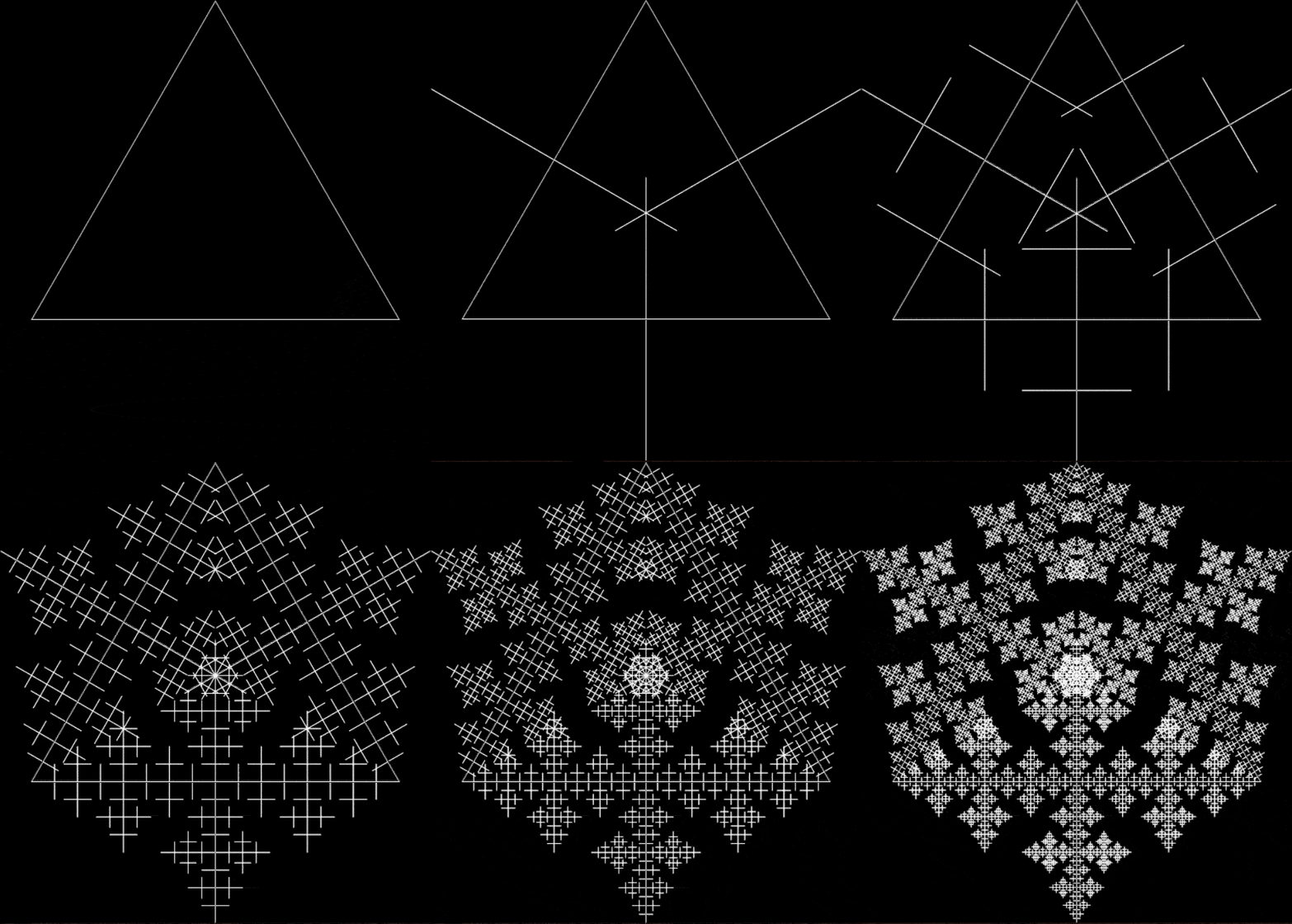
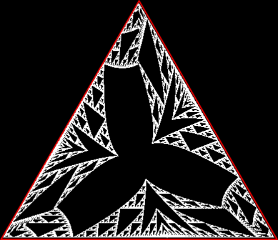
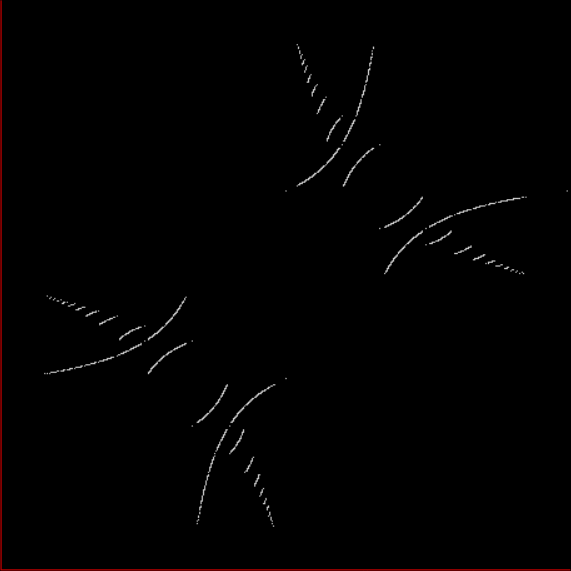
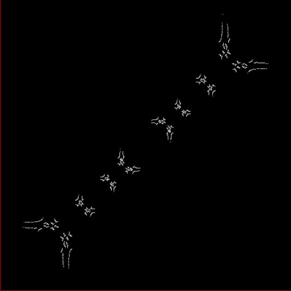
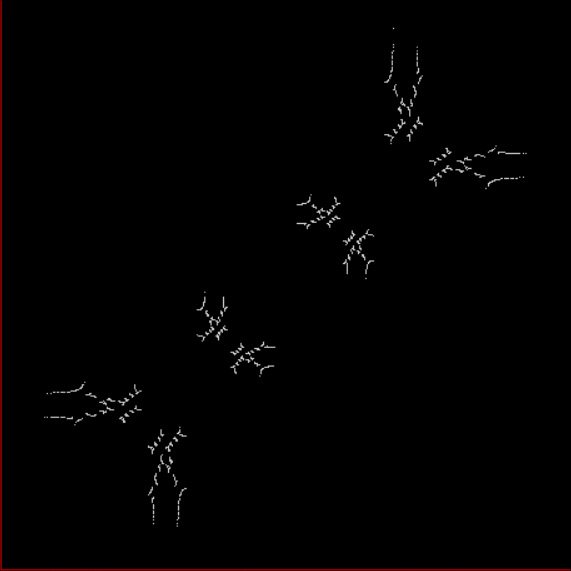
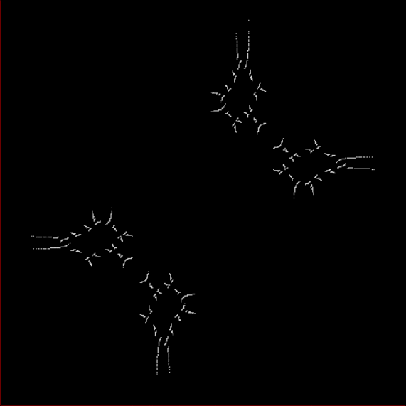
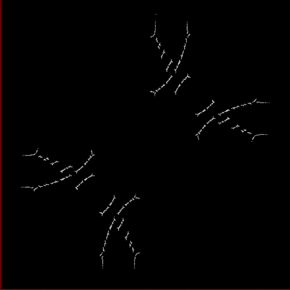
Here’s another variation, what you might call the Koch-Cross flake:

Koch-Cross Flake #0


Koch-Cross Flake #1


Koch-Cross Flake #2


Koch-Cross Flake #3


Koch-Cross Flake #4


Koch-Cross Flake #5


Koch-Cross Flake #6


Koch-Cross Flake #0-6 (animated at ezGif)


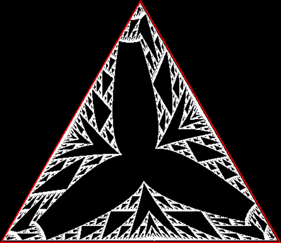
And the Koch-Cross un-flake:

Koch-Cross un-Flake


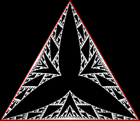
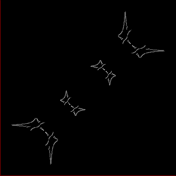
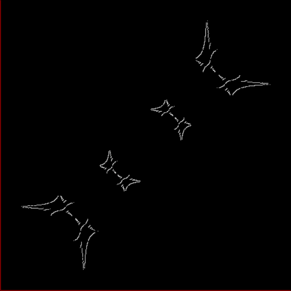
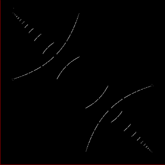
And combined Koch-Cross Flake+un-Flake:

Combined Koch-Cross Flake+un-Flake


Here’s an animation of the combined Koch-Cross Flake+un-Flake:

Combined Koch-Cross Flake+un-Flake (animated at ezGif)


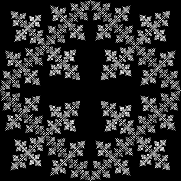
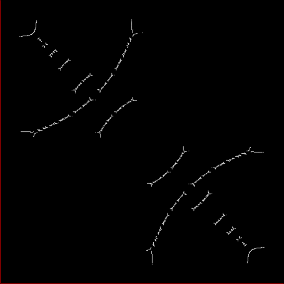
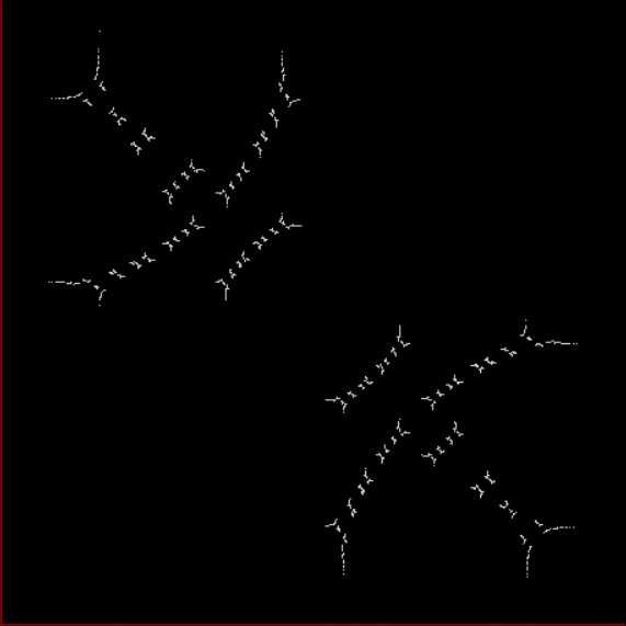
And the combined Koch-Cross Flake+un-Flake created on the sides of a square:

Combined Koch-Cross Flake+un-Flake on square


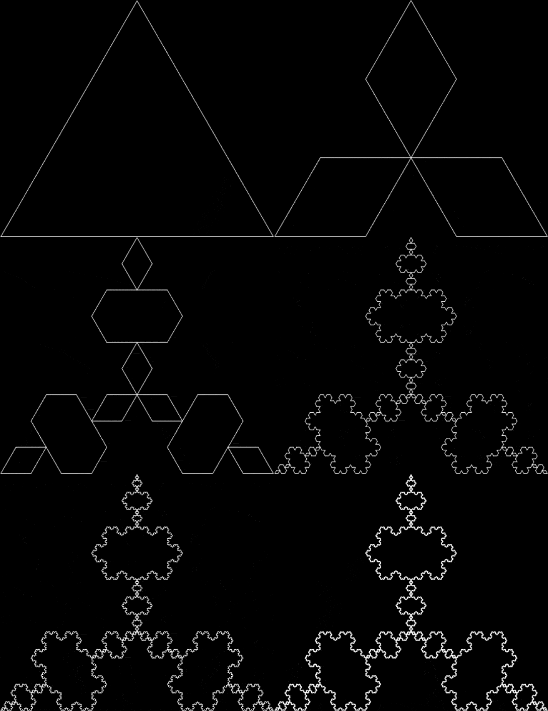
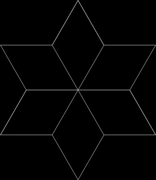
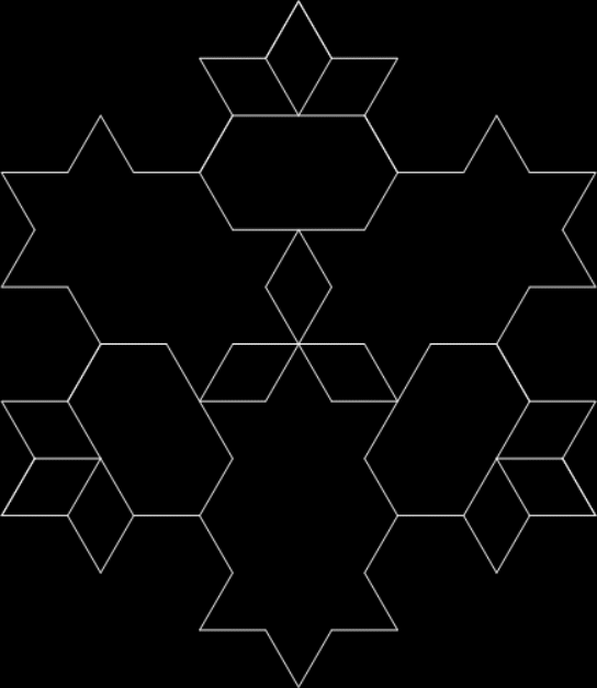
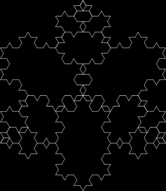
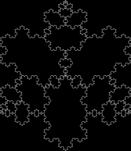
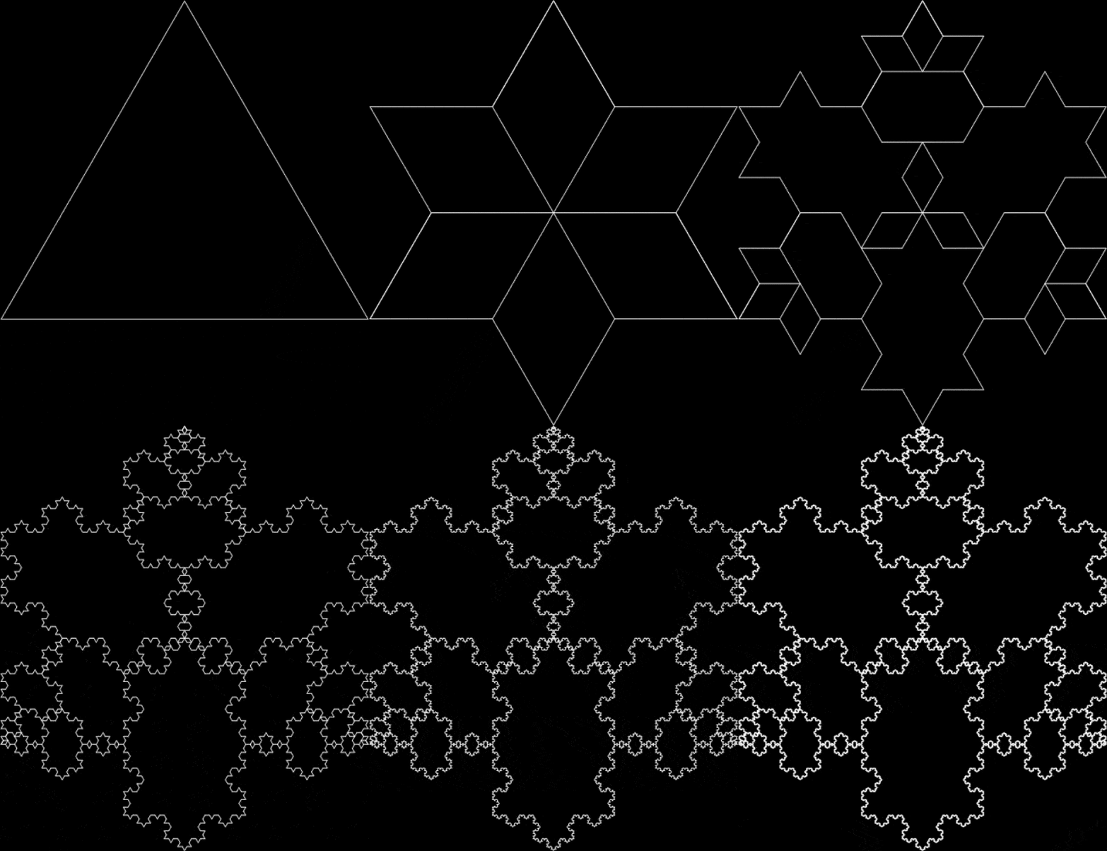
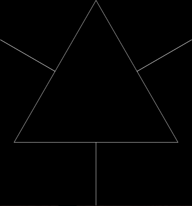
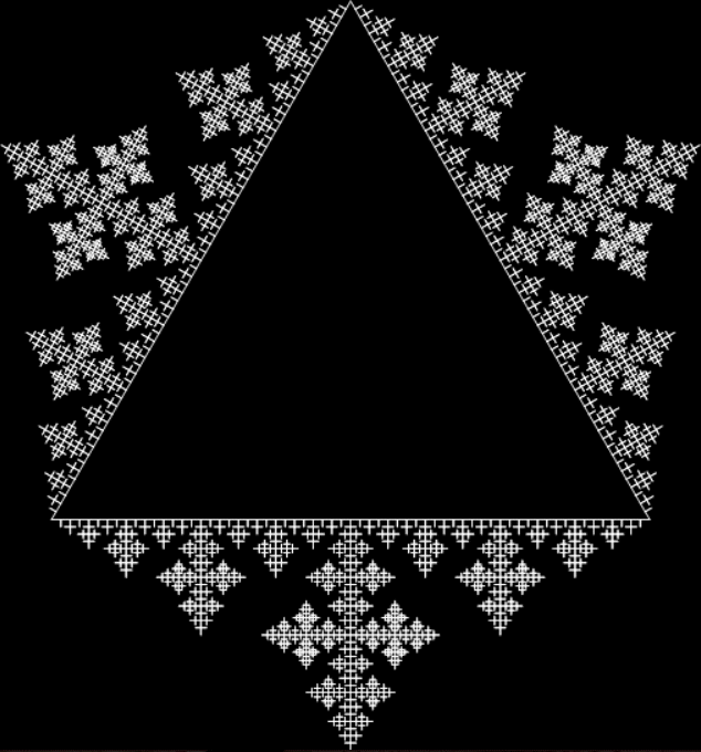
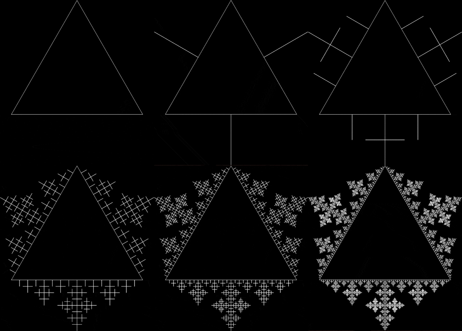
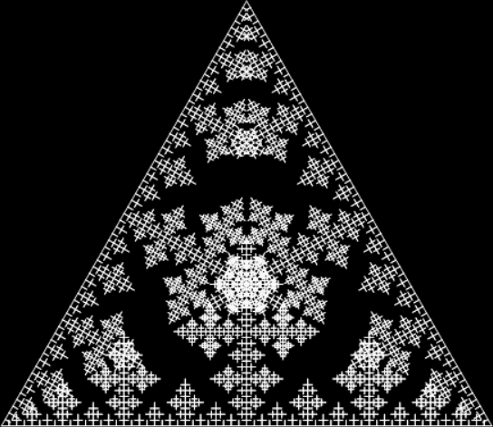
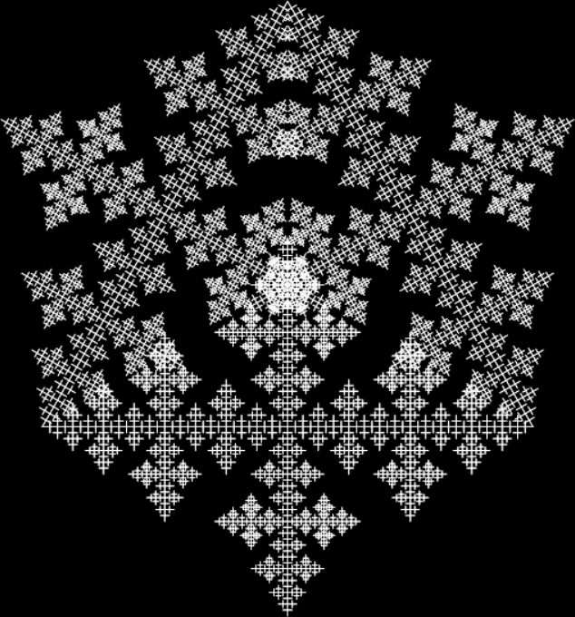
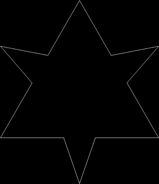
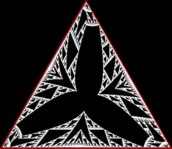
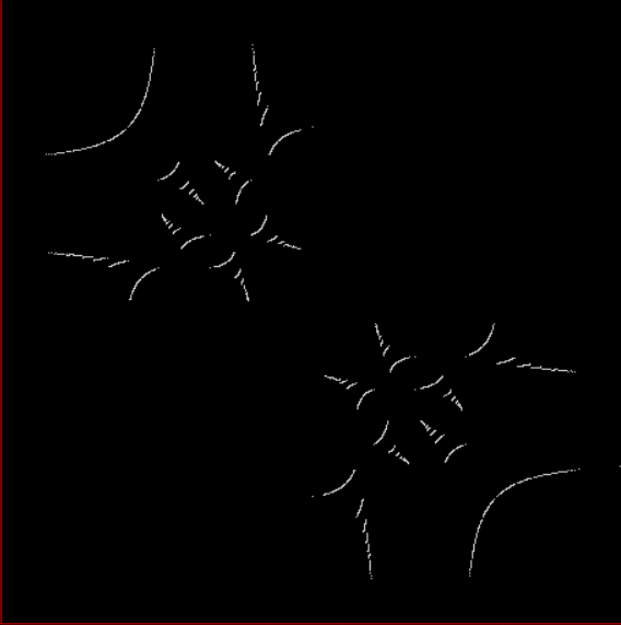
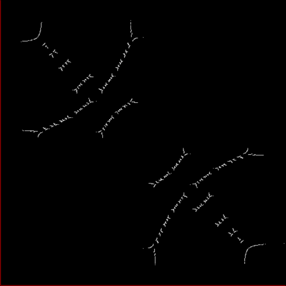
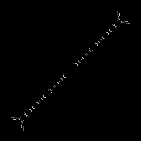
And a final variant of the infinitely many on offer:

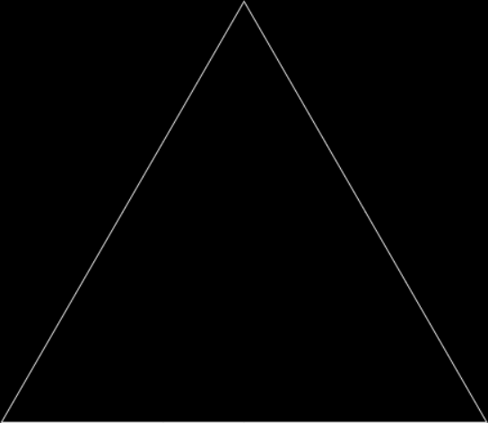
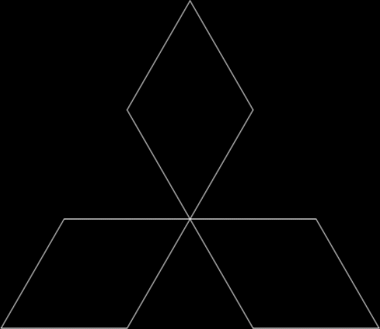
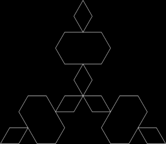
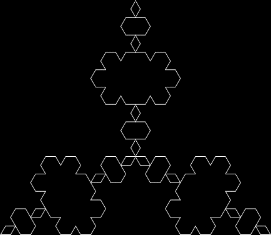
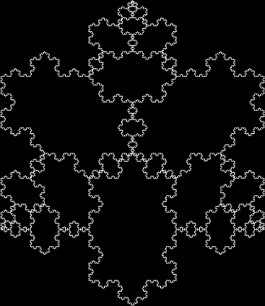
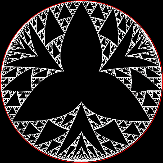
Variant Koch snowflake stage #1


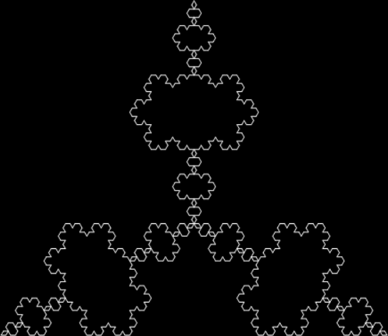
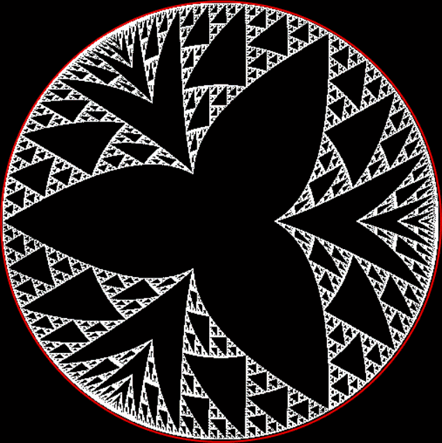
Variant Koch snowflake stage #6


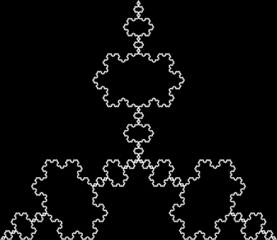
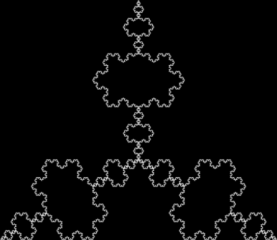
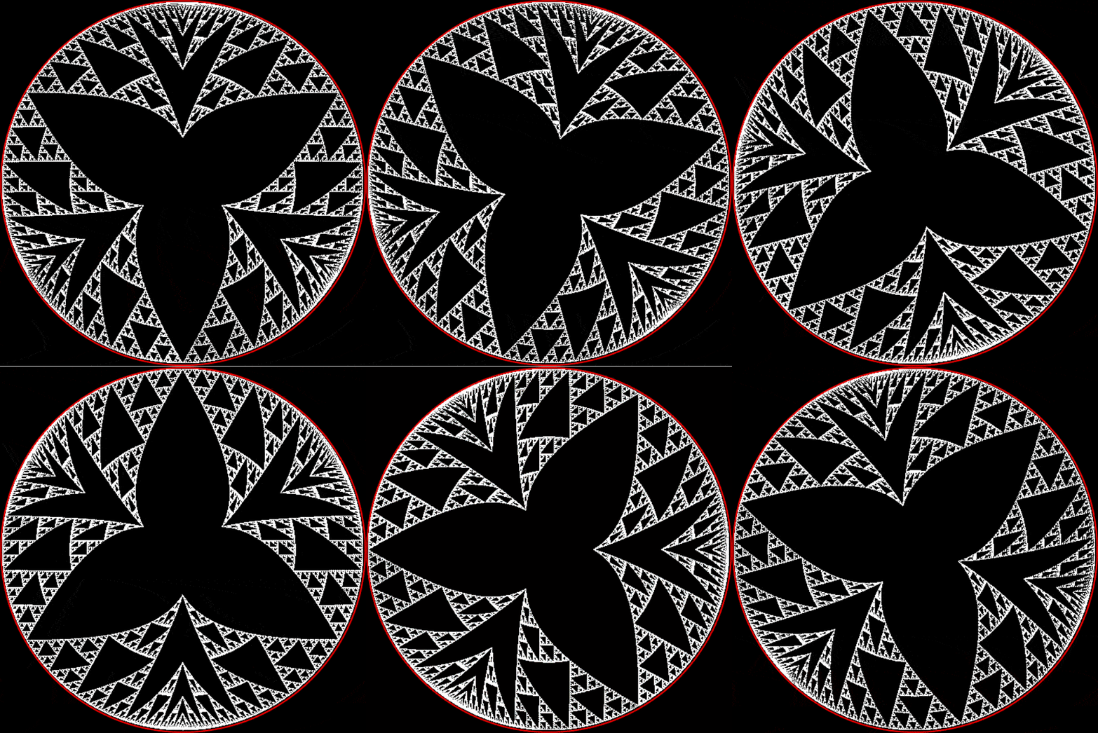
Un-Flake of variant Koch snowflake


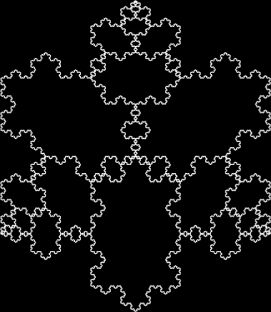
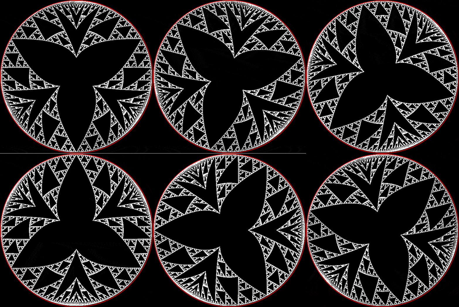
Combined variant Koch Flake+un-Flake


Back in Frac

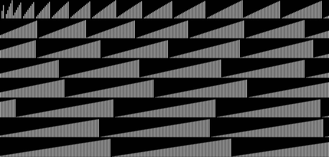
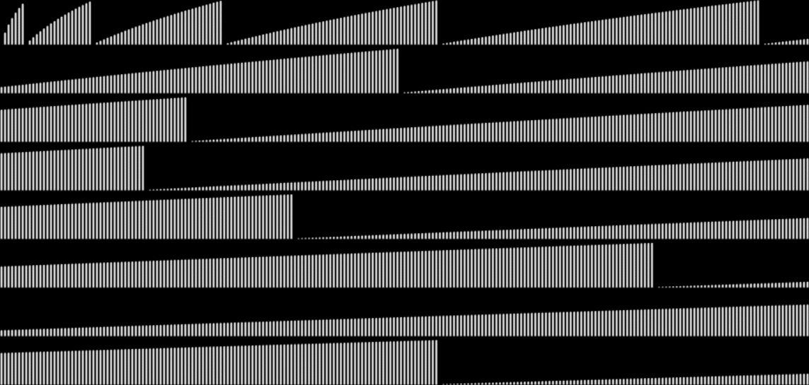
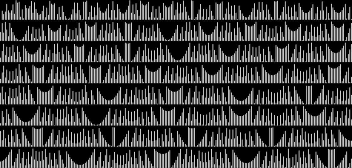
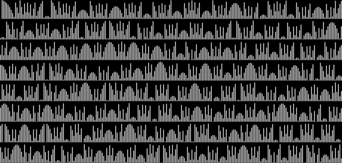
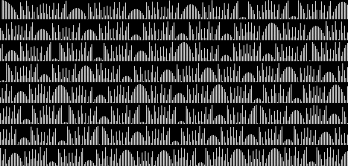
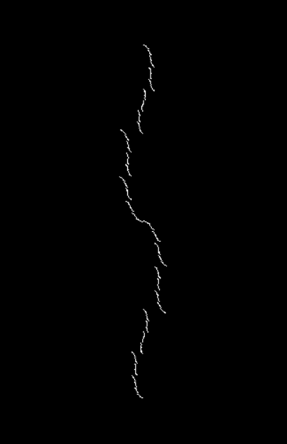
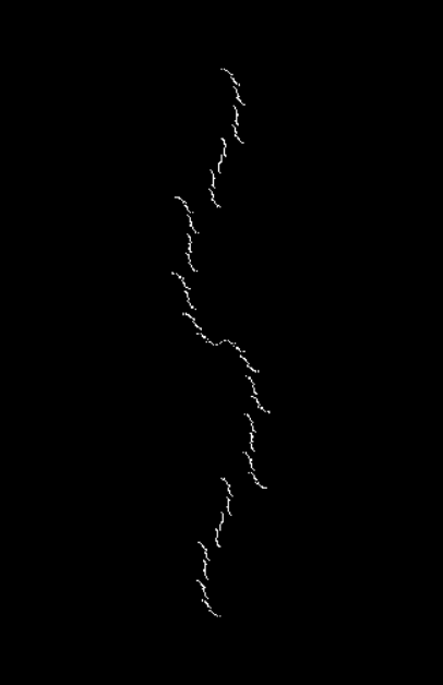
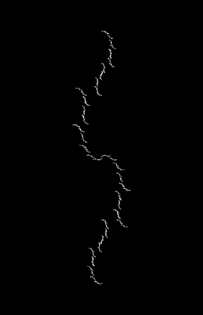
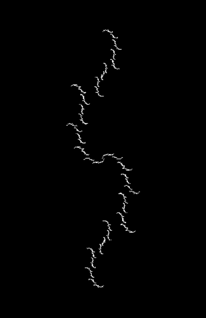
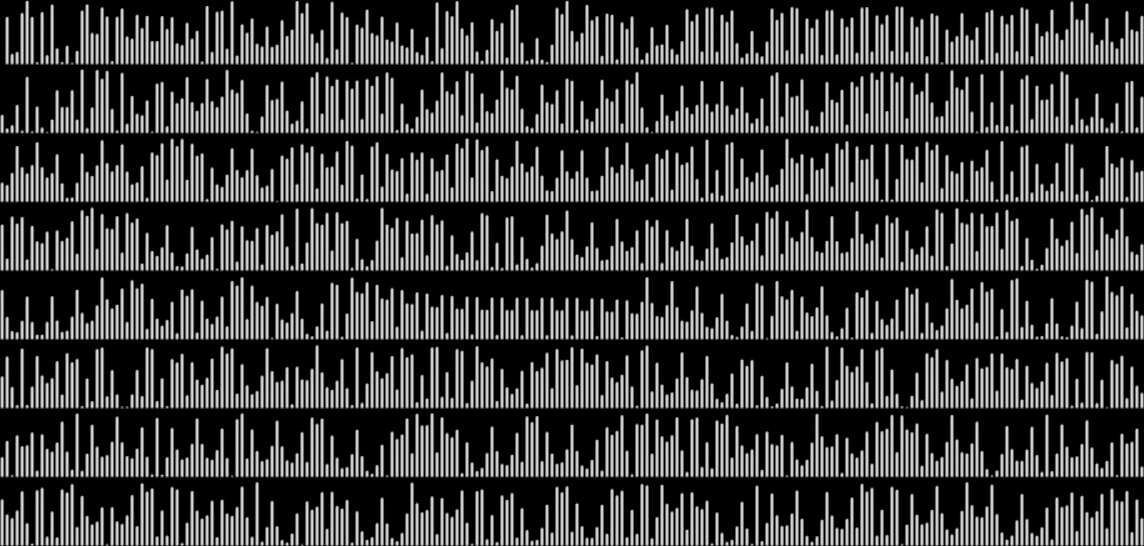
Here’s a graph representing the fractional parts of √n for n = 1 to 1832, with frac(√1) at the top left and frac(√1832) at the bottom right:

graph for frac(√n), n = 1..1832


There’s an odd optical illusion making it seem as though each set of triangular waves ends lower on the right than it starts on the left. Otherwise, it’s a dull graph, because the fractional part of √n simply rises towards 0.9999…, then falls to 0 like this:

0 = frac(1) = frac(√1)
0.414213562373… = frac(1.414213562373…) = frac(√2)
0.732050807568… = frac(1.732050807568…) = frac(√3)
0 = frac(2) = frac(√4)
0.236067977499… = frac(2.236067977499…) = frac(√5)
0.449489742783… = frac(2.449489742783…) = frac(√6)
0.645751311064… = frac(2.645751311064…) = frac(√7)
0.828427124746… = frac(2.828427124746…) = frac(√8)
0 = frac(3) = frac(√9)
0.162277660168… = frac(3.162277660168…) = frac(√10)
0.316624790355… = frac(3.316624790355…) = frac(√11)
0.464101615137… = frac(3.464101615137…) = frac(√12)
0.605551275463… = frac(3.605551275463…) = frac(√13)
0.741657386773… = frac(3.741657386773…) = frac(√14)
0.872983346207… = frac(3.872983346207…) = frac(√15)
0 = frac(4) = frac(√16)
0.123105625617… = frac(4.123105625617…) = frac(√17)
0.242640687119… = frac(4.242640687119…) = frac(√18)
0.358898943540… = frac(4.358898943540…) = frac(√19)
0.472135954999… = frac(4.472135954999…) = frac(√20)

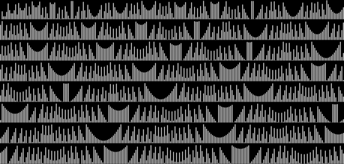
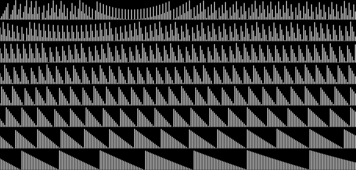
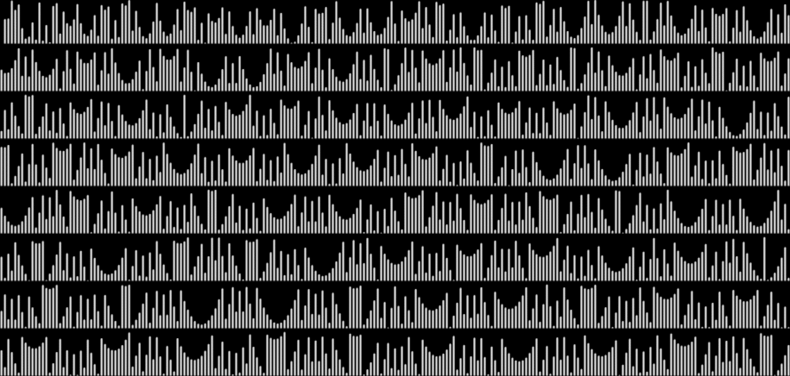
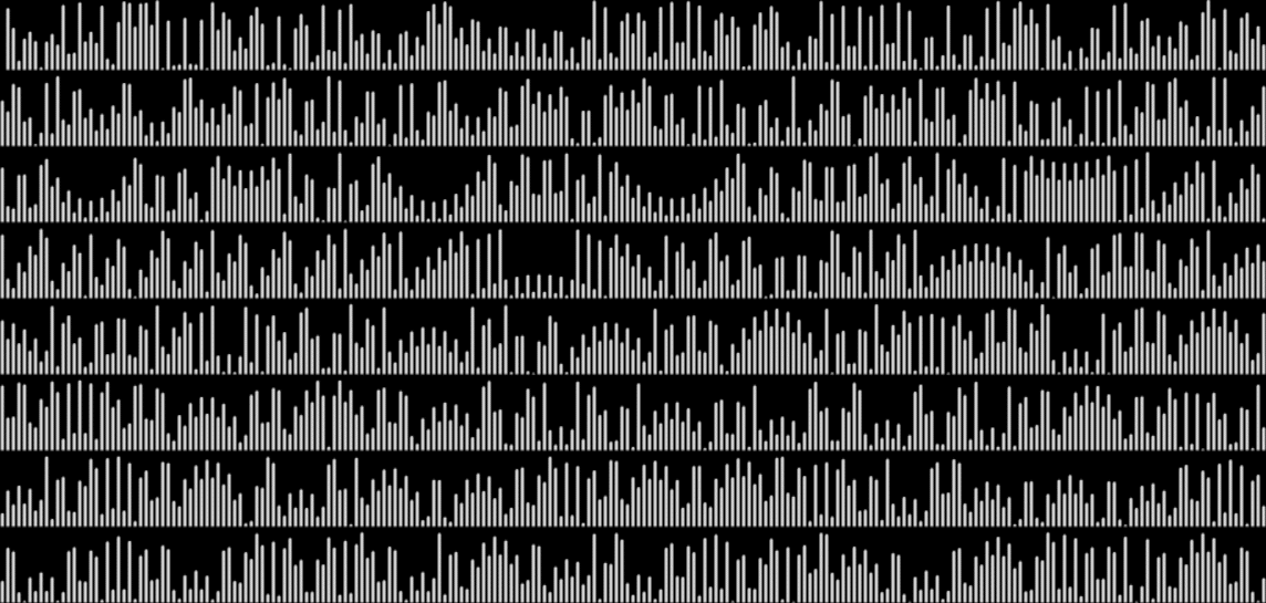
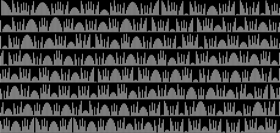
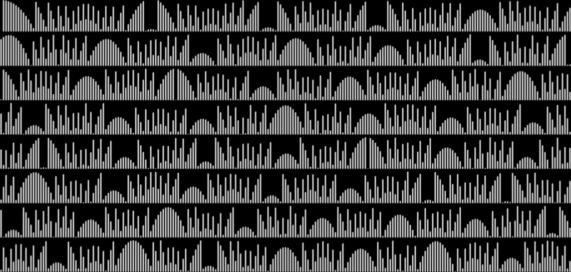
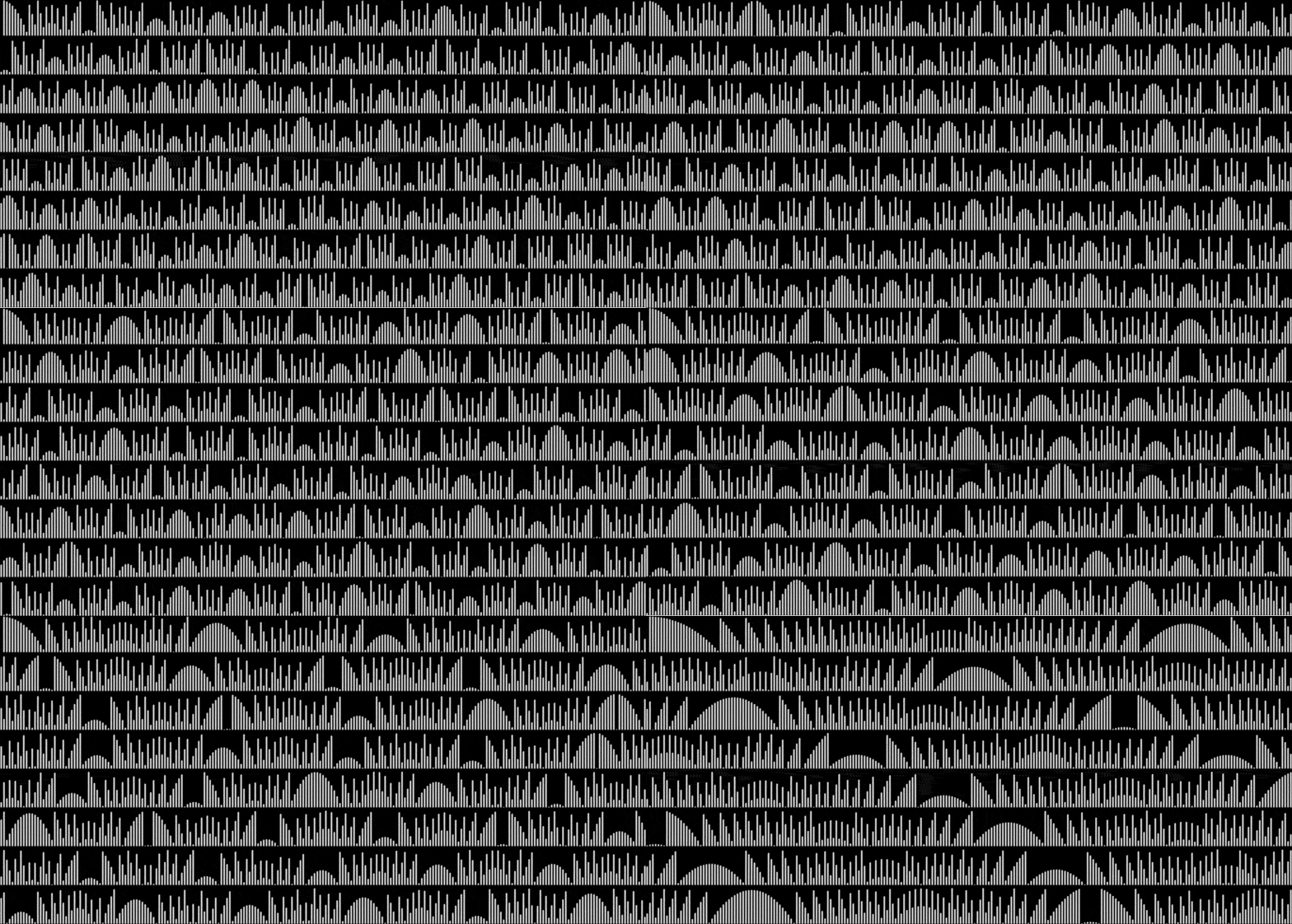
But what about the fractional parts of the sum of √n? What does that graph look like? Much more interesting:

frac(sum(√n)), n = 1..1832


Here are the fractional parts for the sum of √n:

0 = frac(1) = frac(sum(√1))
0.414213562373… = frac(02.414213562373…) = frac(sum(√1..√2))
0.146264369941… = frac(04.146264369941…) = frac(sum(√1..√3))
0.146264369941… = frac(06.146264369941…) = frac(sum(√1..√4))
0.382332347441… = frac(08.382332347441…) = frac(sum(√1..√5))
0.831822090224… = frac(10.831822090224…) = frac(sum(√1..√6))
0.477573401289… = frac(13.477573401289…) = frac(sum(√1..√7))
0.306000526035… = frac(16.306000526035…) = frac(sum(√1..√8))
0.306000526035… = frac(19.306000526035…) = frac(sum(√1..√9))
0.468278186204… = frac(22.468278186204…) = frac(sum(√1..√10))
0.784902976559… = frac(25.784902976559…) = frac(sum(√1..√11))
0.249004591697… = frac(29.249004591697…) = frac(sum(√1..√12))
0.854555867161… = frac(32.854555867161…) = frac(sum(√1..√13))
0.596213253935… = frac(36.596213253935…) = frac(sum(√1..√14))
0.469196600142… = frac(40.469196600142…) = frac(sum(√1..√15))
0.469196600142… = frac(44.469196600142…) = frac(sum(√1..√16))
0.592302225760… = frac(48.592302225760…) = frac(sum(√1..√17))
0.834942912879… = frac(52.834942912879…) = frac(sum(√1..√18))
0.193841856420… = frac(57.193841856420…) = frac(sum(√1..√19))
0.665977811419… = frac(61.665977811419…) = frac(sum(√1..√20))

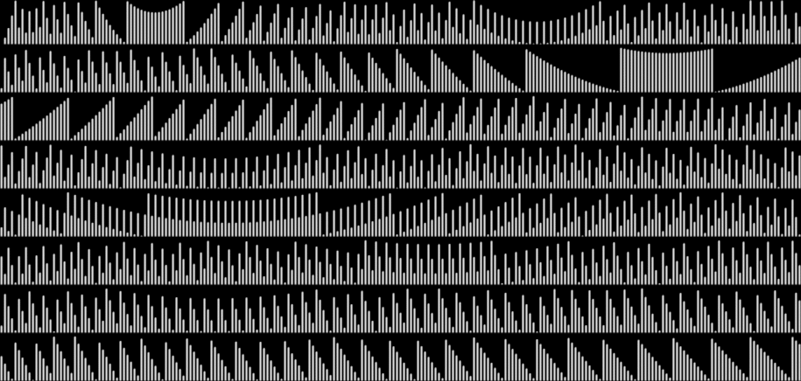
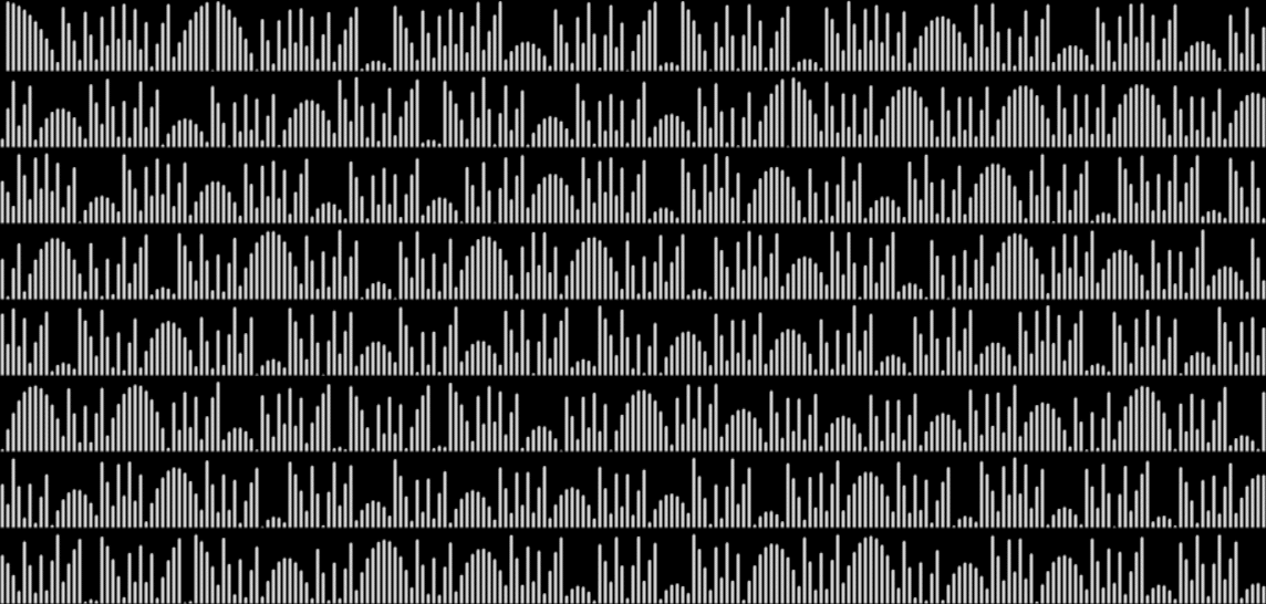
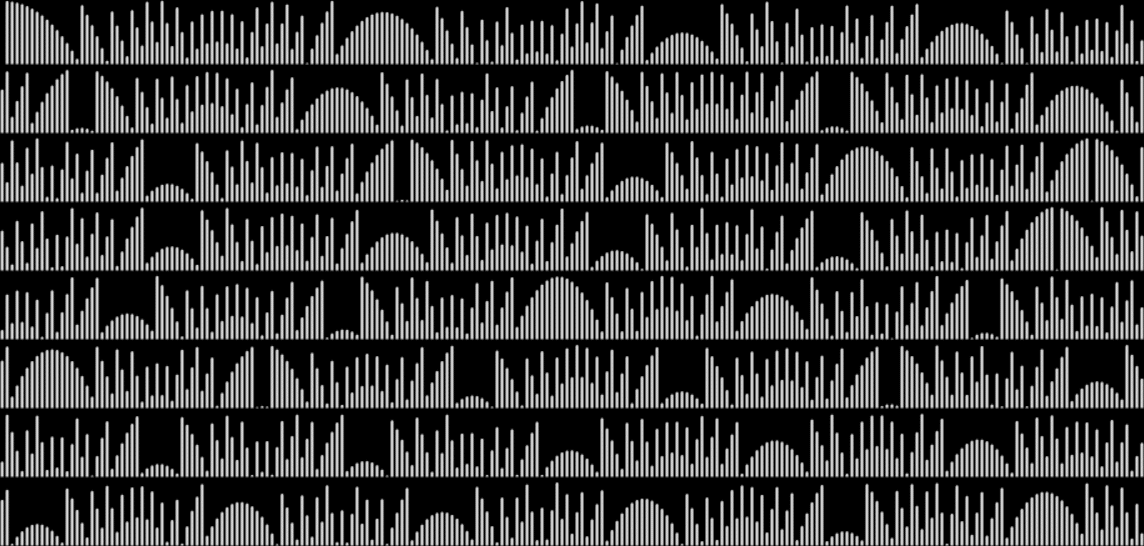
As with square roots, so with cube roots. The graph of frac(∛n) looks like this:

frac(∛n), n = 1..1832


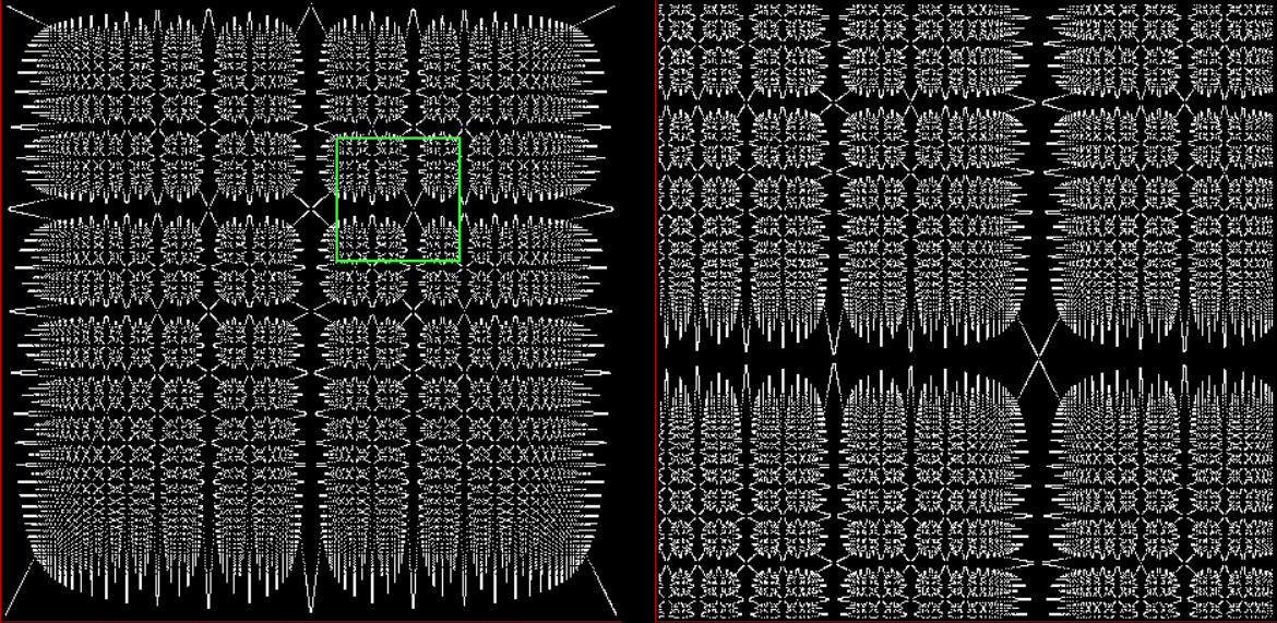
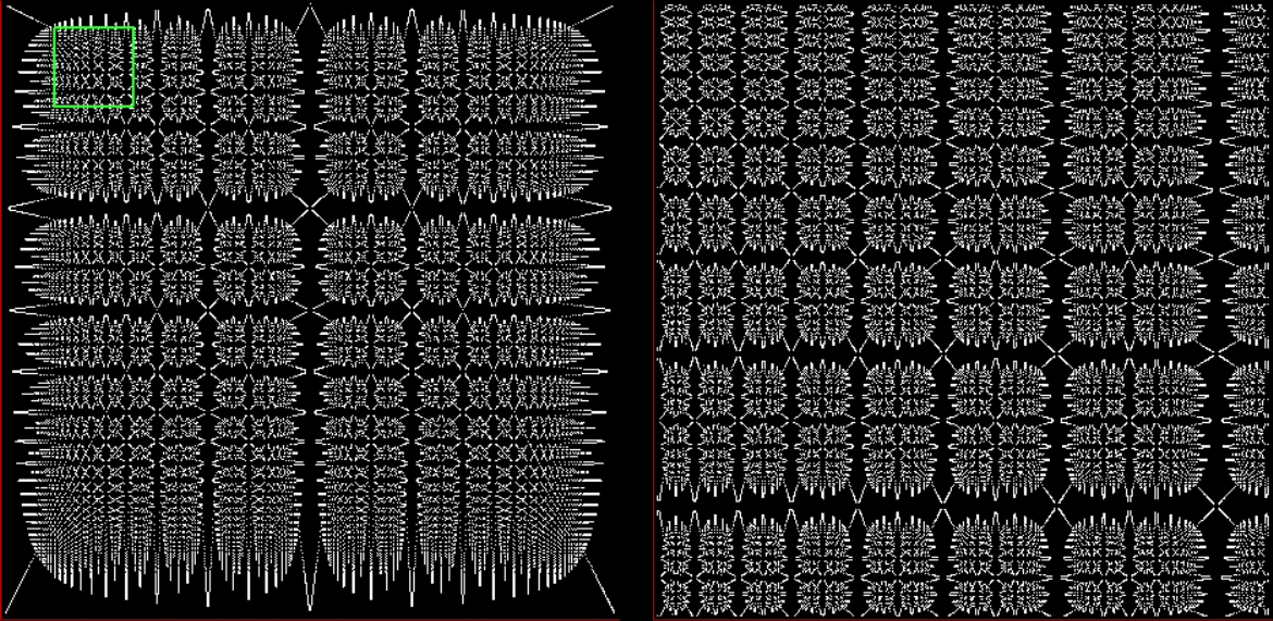
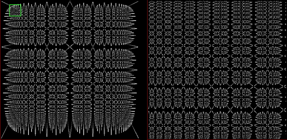
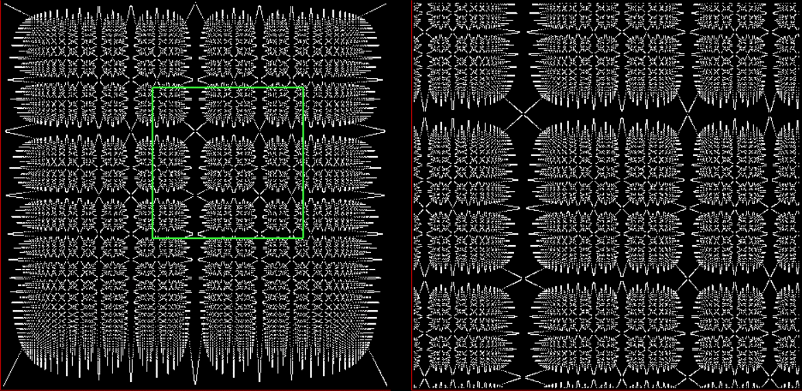
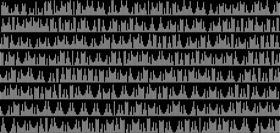
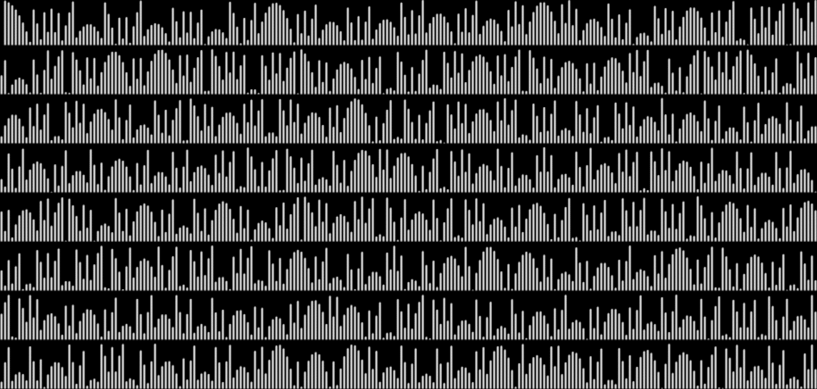
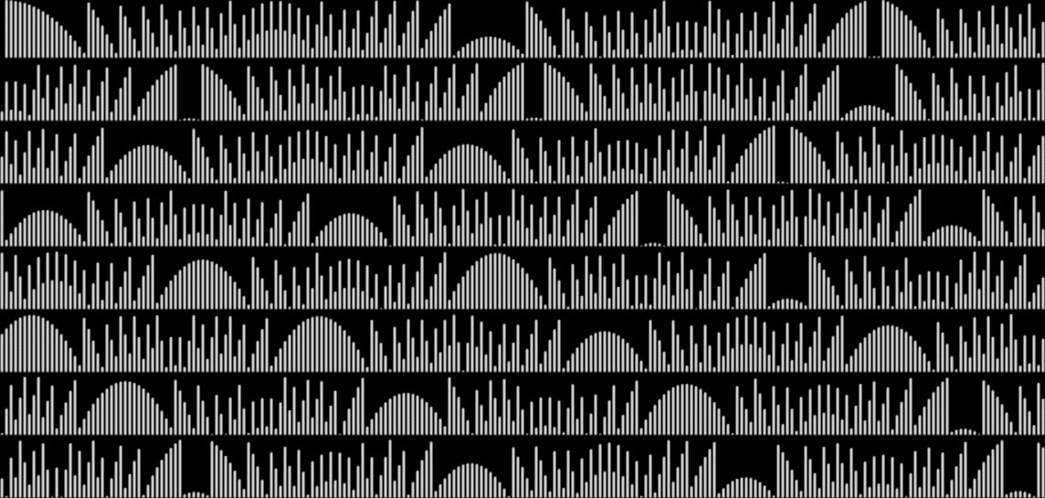
It’s dull again, because the fractional part of ∛n is simply rising towards 0.9999…, then falling to 0. Just more slowly. But the graph of frac(sum(∛n)) looks like this:

frac(sum(∛n))


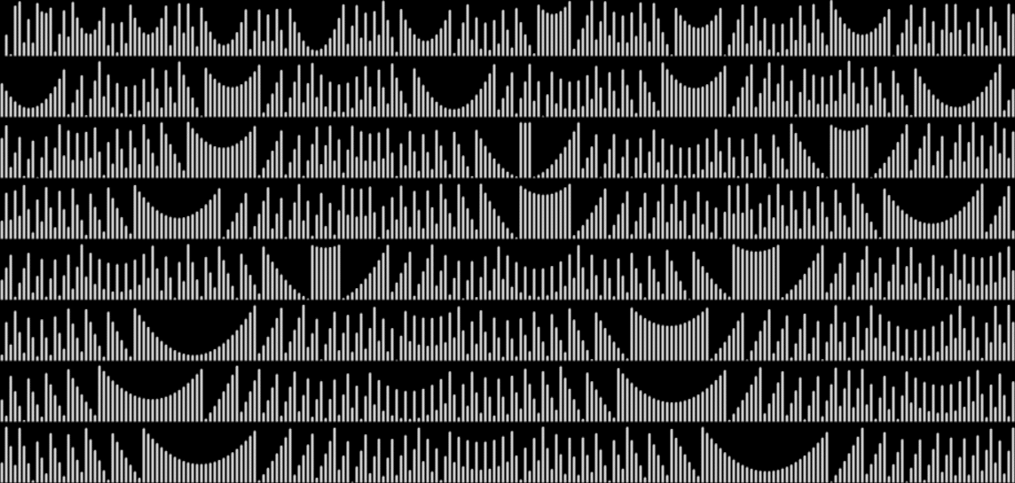
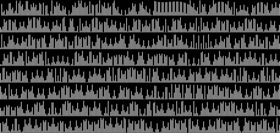
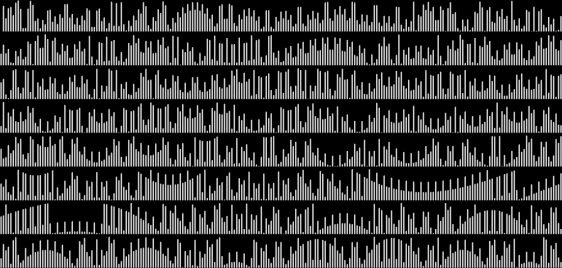
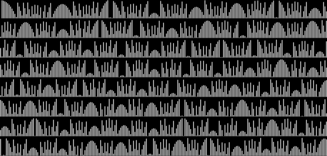
But roots don’t end with √n and ∛n, of course. Those roots represent n^(1/2) and n^(1/3), respectively, because when x = n^(a/b), n = x^(b/a). What about the graph of sum(n^(4/5)), where n = (n^4/5)^(5/4)? The graph looks like this:

frac(sum(n^(4/5)))


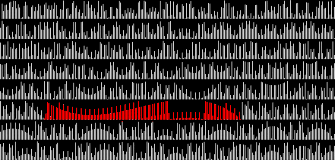
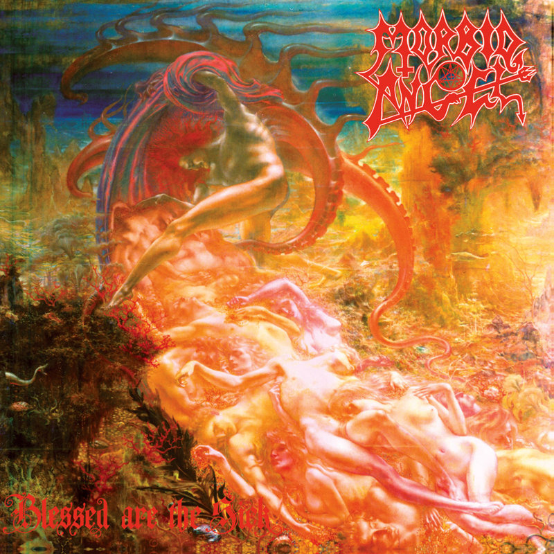
One of the curves in that graph reminds of the cephalopodic tentacles in Jean Delville’s marvellous painting Les Trésors de Sathan (sic) (Treasures of Satan) (1895), which was used on the cover of Morbid Angel’s Blessed Are the Sick (1991). The curve is longer in frac(sum(n^(84/97))):

frac(sum(n^(84/97))) (curve in red)


Les Trésors de Sathan (1895) by Jean Delville as the cover of Blessed Are the Sick (1991)


frac(sum(n^(4/5))) (curve in red)


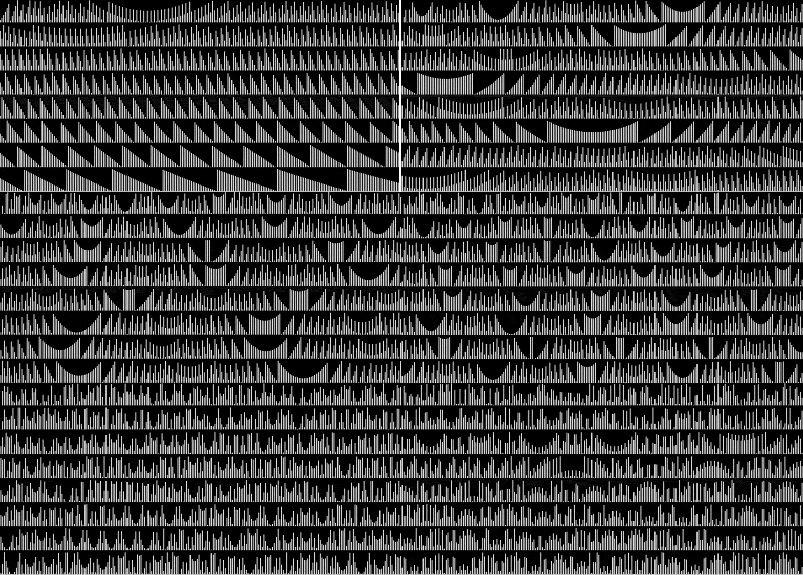
Those Delvillean curves are examples of how, as the a/b of n^(a/b) climbs from 1/b to (b-1)/b, the graph of frac(sum(n^(a/b))) changes in interesting ways. Here are the graphs for n^(1..10/11):

frac(sum(n^(1/11)))


frac(sum(n^(2/11)))


frac(sum(n^(3/11)))


frac(sum(n^(4/11)))


frac(sum(n^(5/11)))


frac(sum(n^(6/11)))


frac(sum(n^(7/11)))


frac(sum(n^(8/11)))


frac(sum(n^(9/11)))


frac(sum(n^(10/11)))


Here’s an animation of those graphs:

animation of frac(sum(n^(1/11..10/11))) (created at ezGif)


And here are graphs for n^(72/83) and n^(82/83), with a Delvillean curve in the graph of 72/83 and domes in the graph of 82/83:

frac(sum(n^(72/83)))


frac(sum(n^(82/83)))


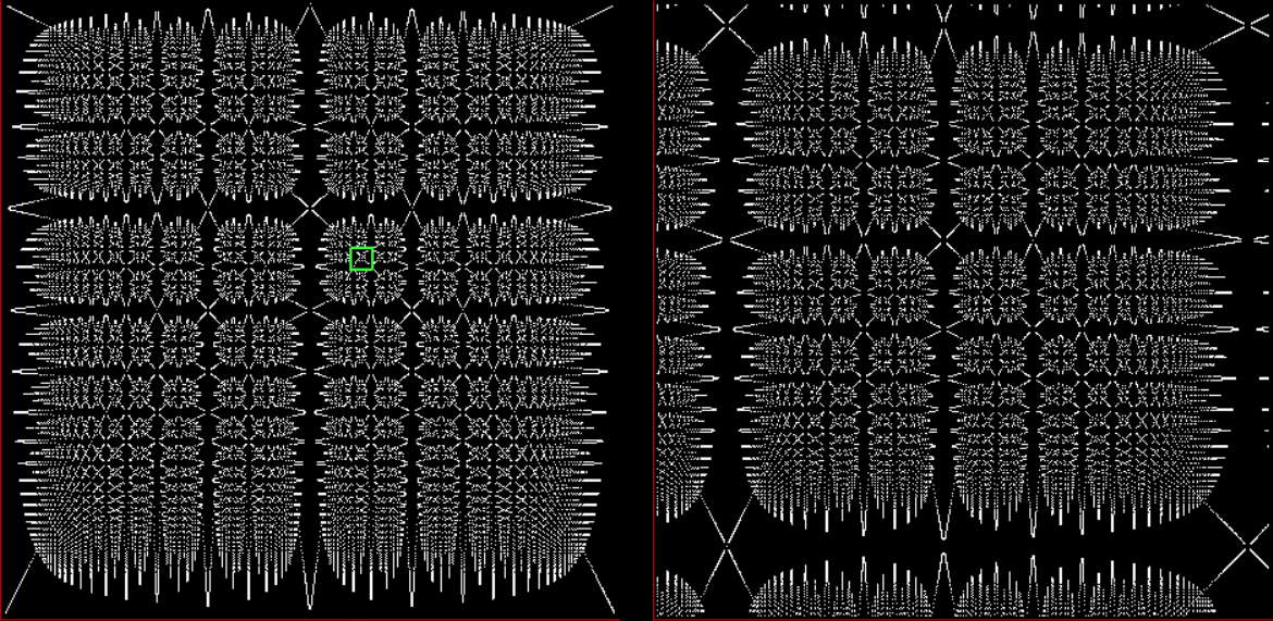
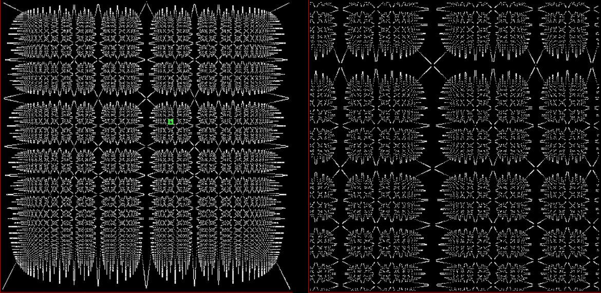
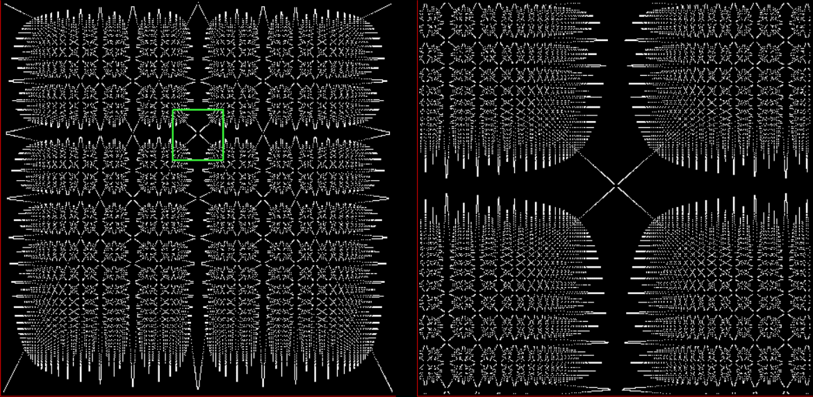
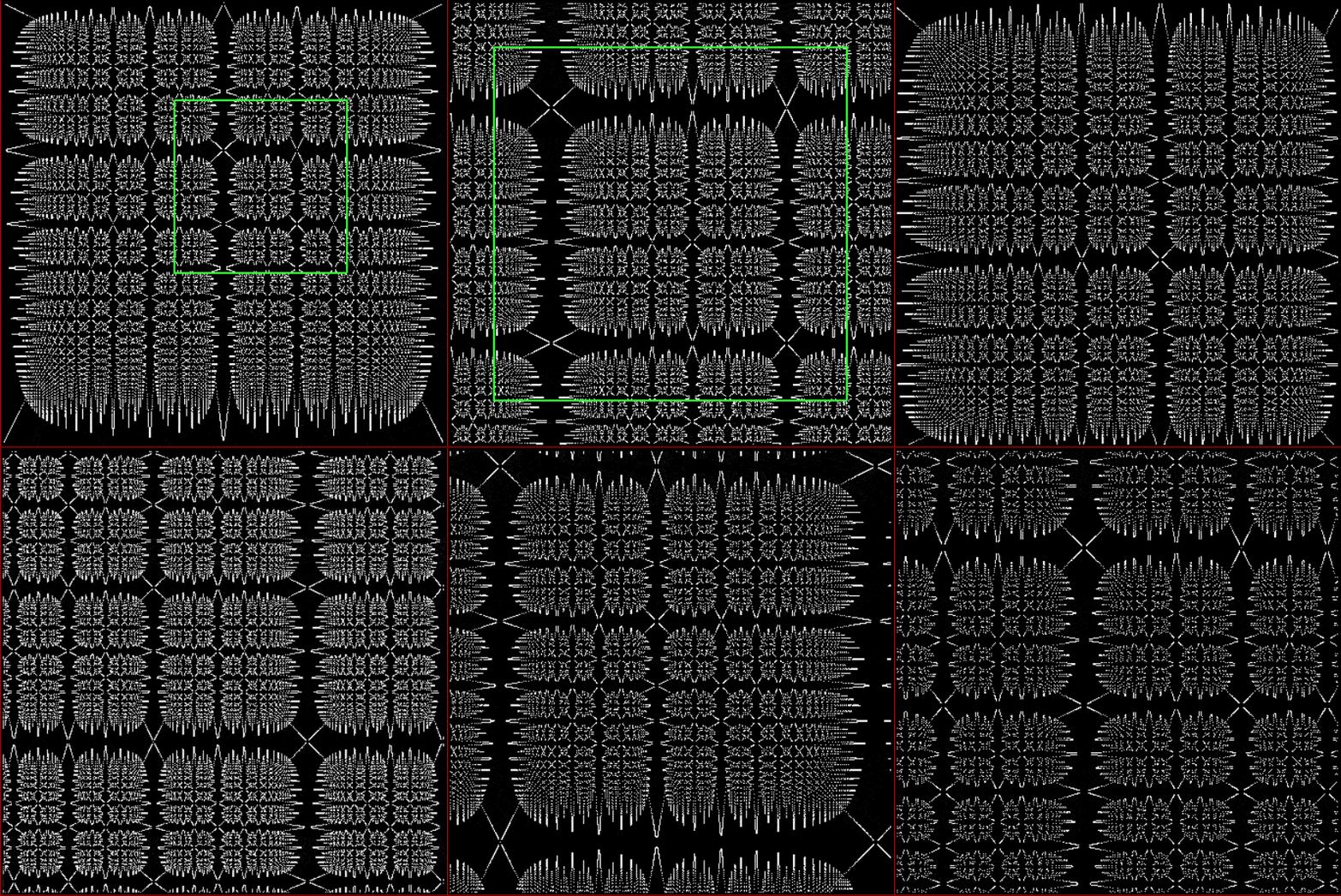
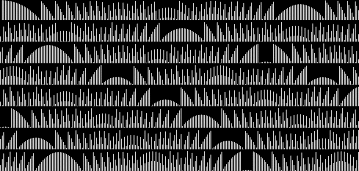
As the denominators get bigger, so do the domes:

frac(sum(n^(1000/1009)))


frac(sum(n^(1001/1009)))


frac(sum(n^(1002/1009)))


frac(sum(n^(1003/1009)))


frac(sum(n^(1004/1009)))


frac(sum(n^(1005/1009)))


frac(sum(n^(1006/1009)))


frac(sum(n^(1007/1009)))


frac(sum(n^(1008/1009)))


Here’s an animation of those graphs:

animation of frac(sum(n^(1000/1009..1008/1009))) (created at ezGif)


Previously Pre-Posted…

• Think Frinc — an earlier look at fraction-patterns
• Altars of Mathness — and similar patterns from integer-digits


Elsewhere Other-Accessible…

• Jean Delville at Wikipedia
• Blessed Are the Sick at BandCamp

Fungible Fractals

Thinking it over, I’ve decided that trircle is a much better name than ciangle:

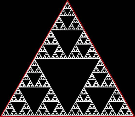
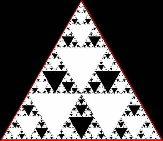
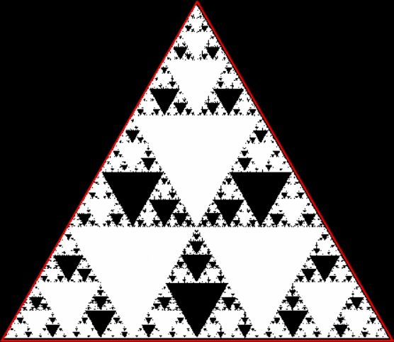
A Sierpiński triangle

↓

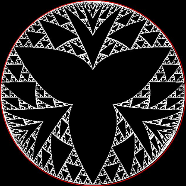
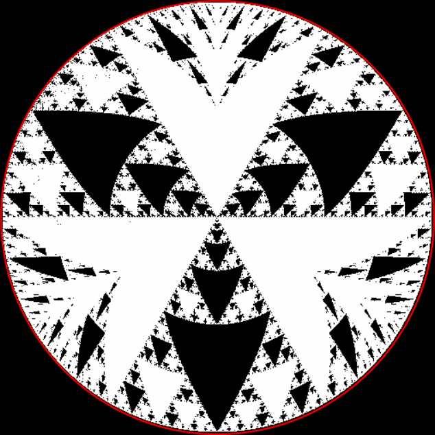
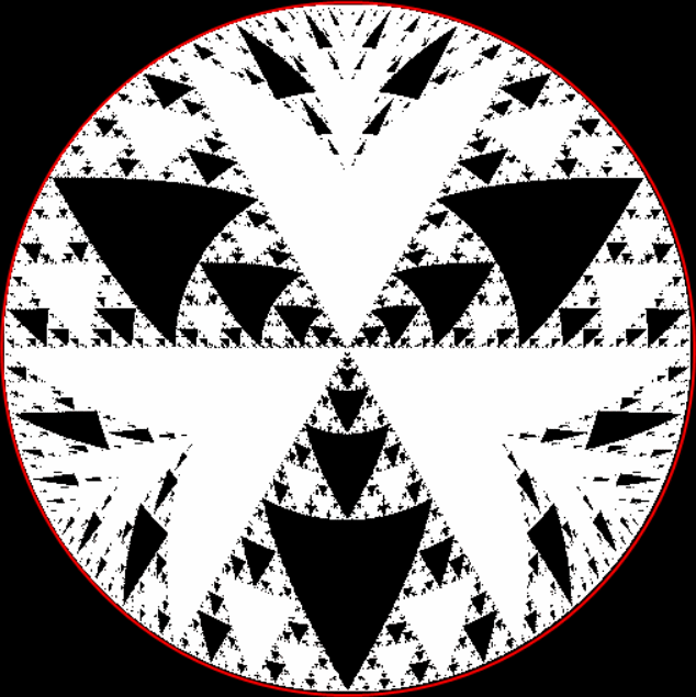
A Sierpiński trircle, or triangle converted into a circle


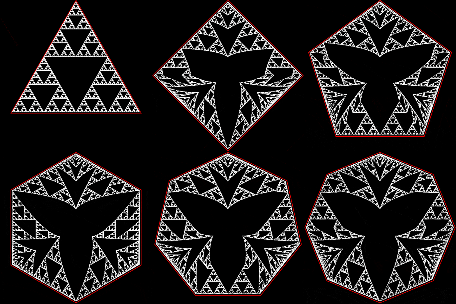
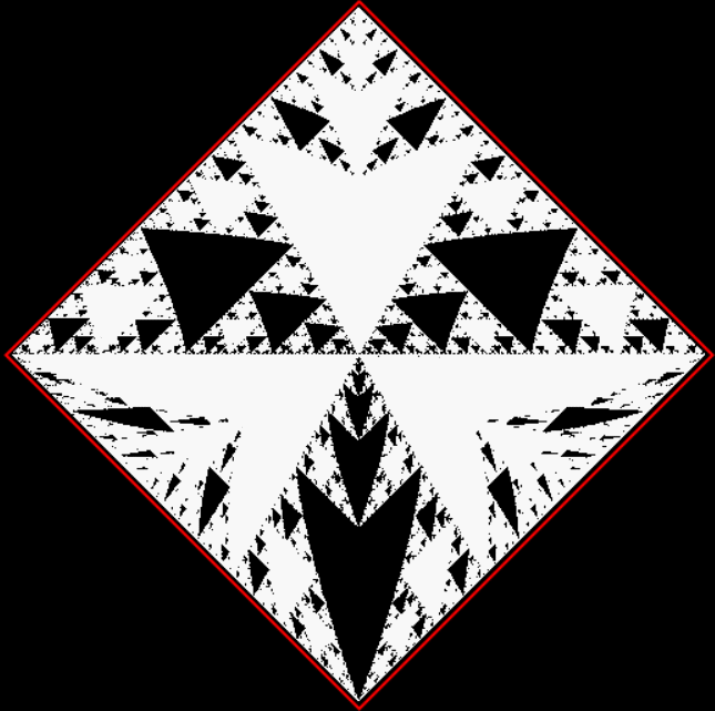
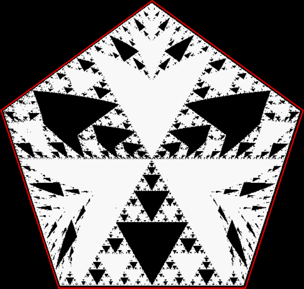
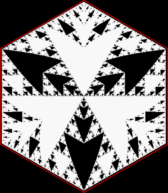
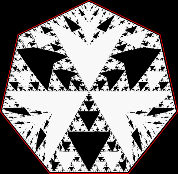
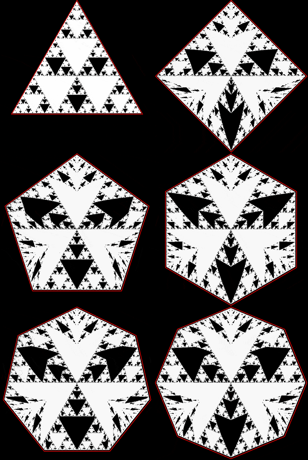
A trircle is a triangle converted into a circle; a ciangle is a circle converted into a triangle. Or another regular polygon. The trircle reminded me that circularized fractals are fungible, because the Sierpiński triangle can be converted into another regular polygon like a square or pentagon or hexagon. You can go viâ the trircle, but you don’t have to. The point is that the Sierpiński triangle has a center and points lying at some distance and some angle 0° through 360°, so you can easily adjust the points to fit inside any other regular polygon:

A Sierpiński triangle again

↓

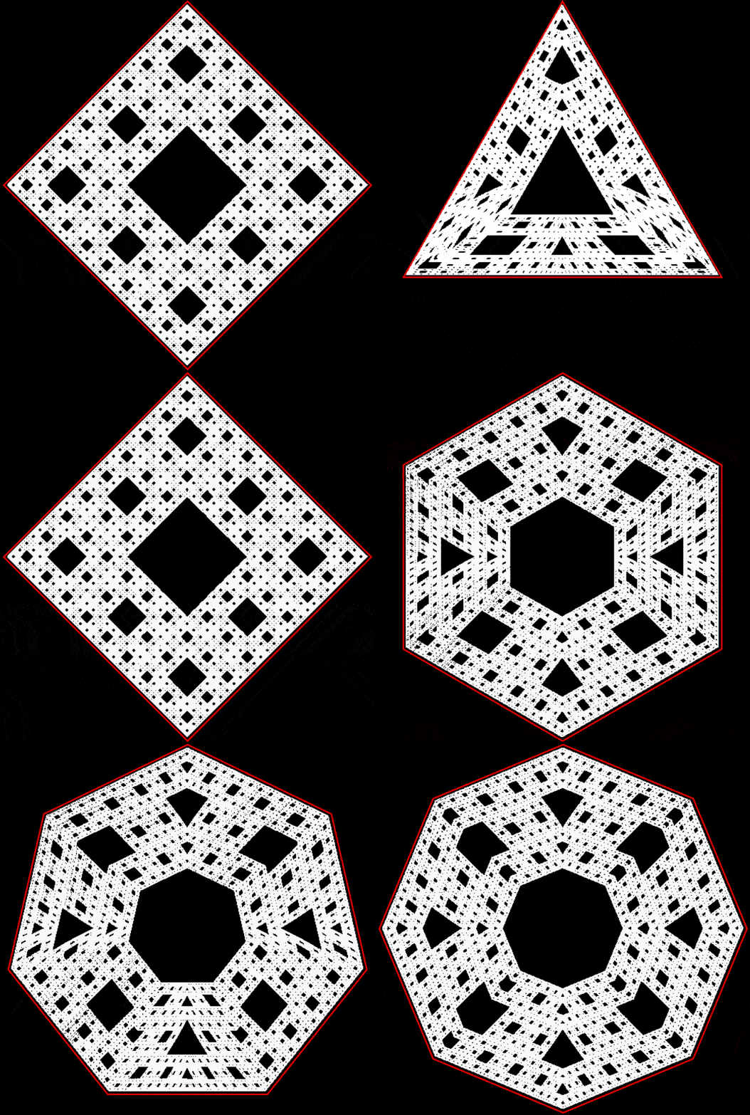
A Sierpiński trare, or triangle converted into square

↓

A Sierpiński trentagon

↓

A Sierpiński trexagon

↓

A Sierpiński treptagon

↓

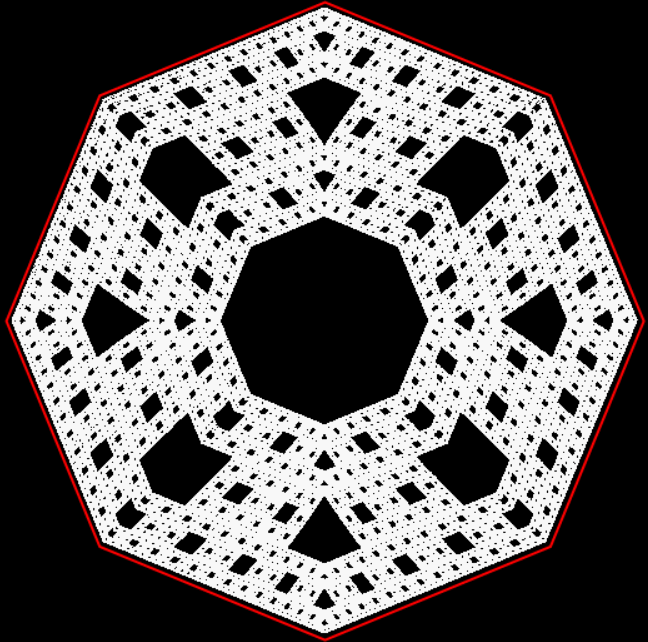
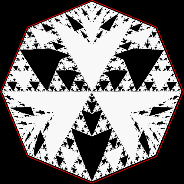
A Sierpiński troctogon


Here’s an animation of the conversions:

Sierpiński triangle → square, pentagon, hexagon, heptagon, octagon (animated at ezGif)


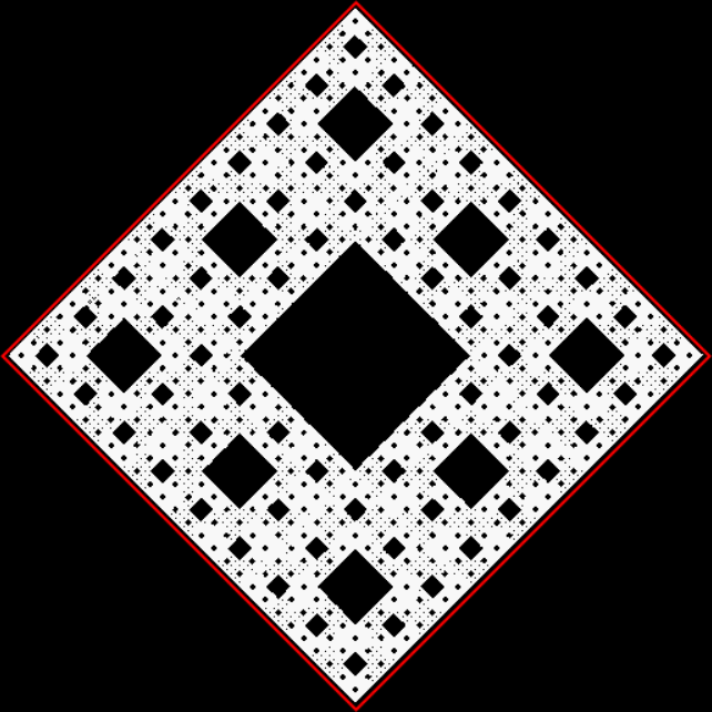
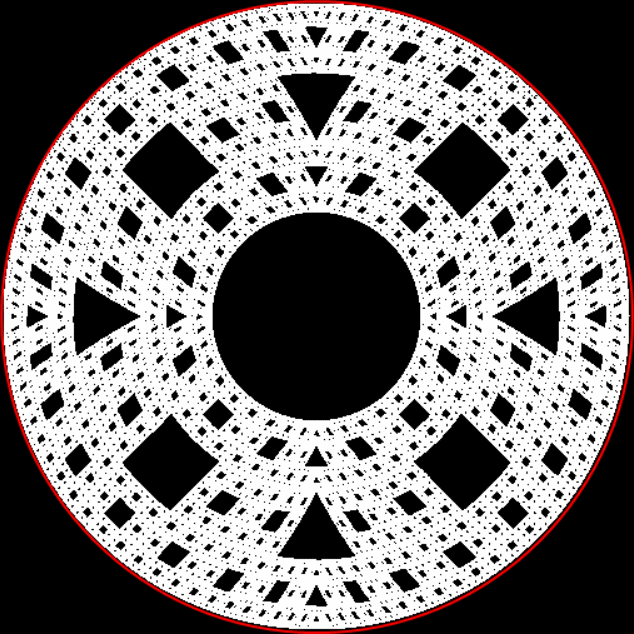
A Sierpiński carpet, with points lying at 0° through 360° inside a square, is similarly fungible:

A Sierpiński carpet

↓

A Sierpiński carpet converted into a circle

↓

A Sierpiński carpet converted into a triangle

↓

A Sierpiński carpet again

↓

A Sierpiński carpet converted into a pentagon

↓

↓

↓


And an animation of the carpet conversions:

Sierpiński carpet → triangle, pentagon, hexagon, heptagon, octagon (animated at ezGif)


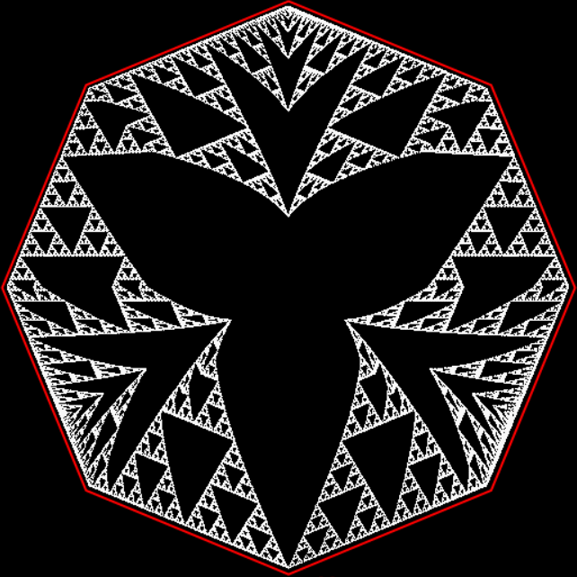
Finally, and fungibly, the fractal that I call the centered Sierpiński triangle:

A centered Sierpiński triangle

↓

A centered Sierpiński trircle, or triangle converted into a circle

↓

↓

↓

↓

↓


And the final animation:

Centered Sierpiński triangle → square, pentagon, hexagon, heptagon, octagon (animated at ezGif)


Flowly We Rote

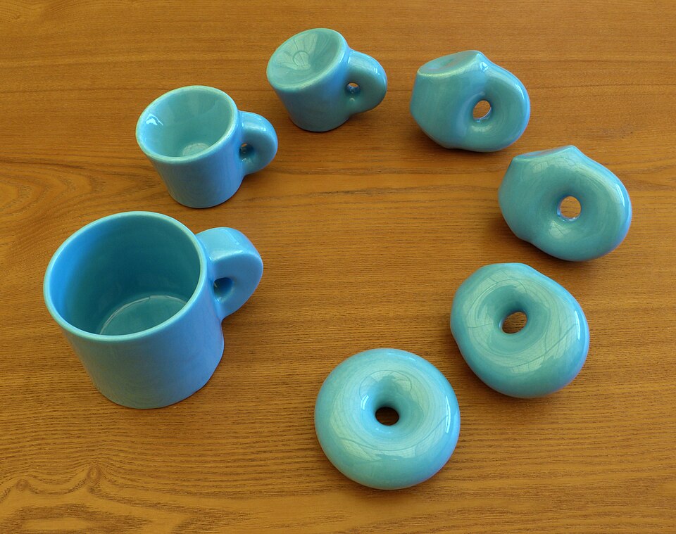
As the old mathematical joke goes: A topologist is someone who can’t tell the difference between a coffee-cup and a donut. That’s because topology is, crudely speaking, the branch of geometry that studies shapes when the distance and angle between one part and another doesn’t matter. For example, how can (or can’t) shapes flow smoothly into each other, without being cut or torn or pierced? The shape of a perfectly plastic substance can flow smoothly from that of a coffee-cup into that of a donut. And vice versa:

Topologically speaking, a coffee-cup is the same as a donut (Wikipedia)


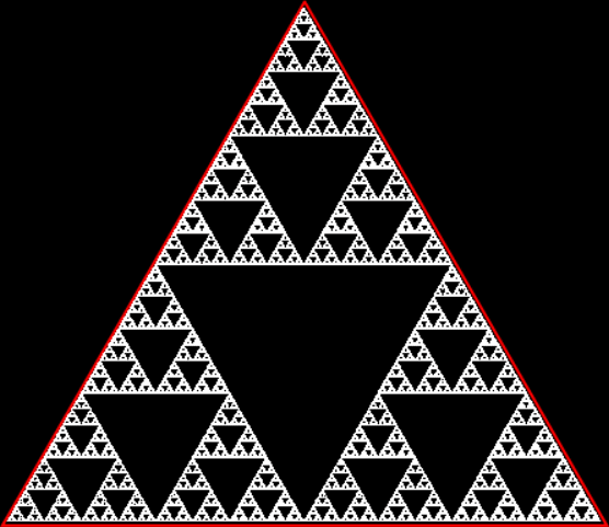
That’s topology in three dimensions. I came across some unexpected topology in two dimensions when I was looking at transformations of a triangle — the Sierpiński triangle, a fractal named after the Polish mathematician Wacław Sierpiński (1882-1969):

Sierpiński triangle


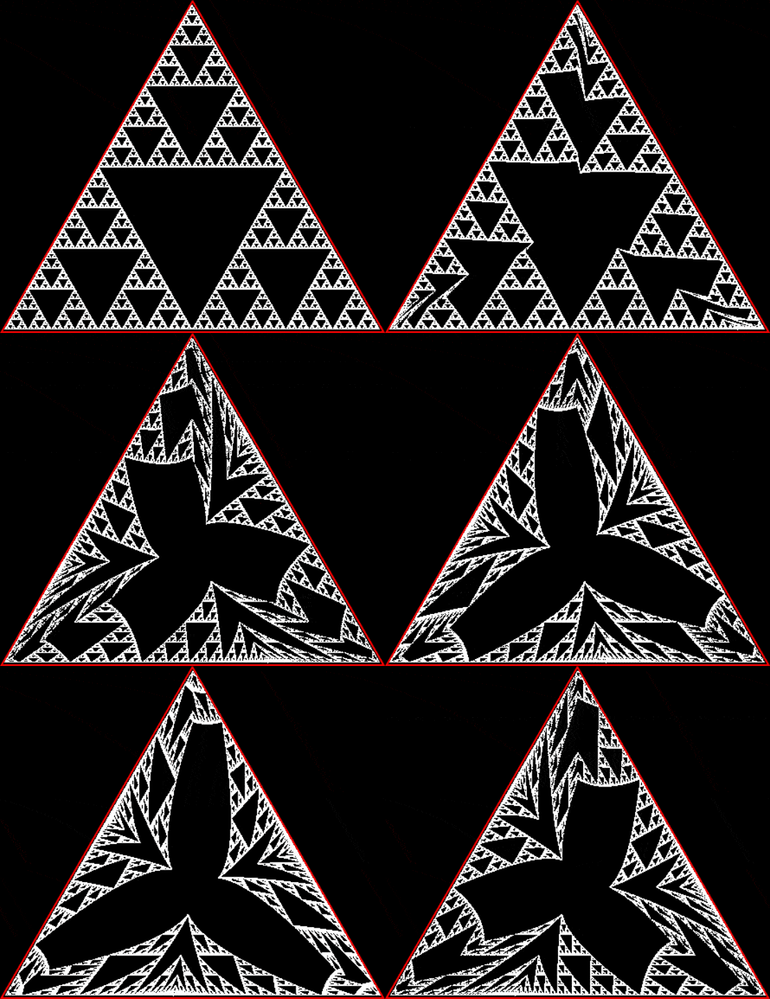
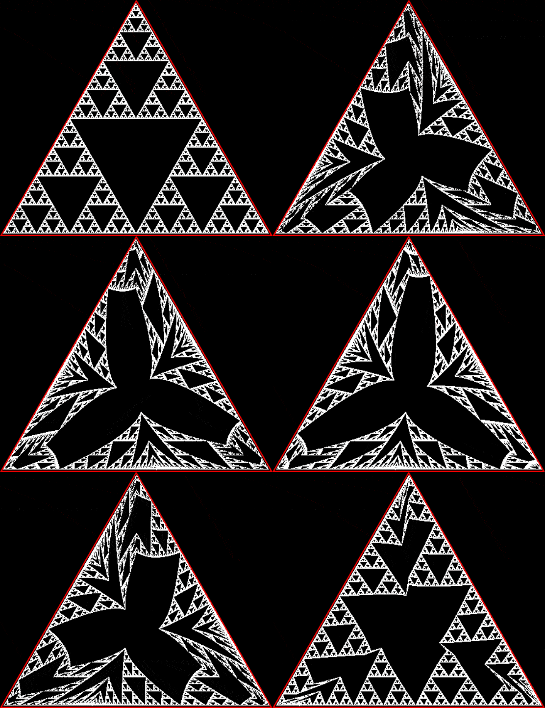
I wondered what happened when you rotate the points inside a Sierpiński triangle while the triangular boundary remains fixed. That is, each point stays at the same position in the width between the center and the boundary as the whole interior flows around the center of the triangle:

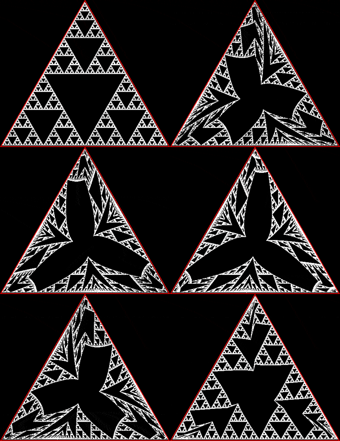
Points inside a Sierpiński triangle rotated by 1°


Points inside a Sierpiński triangle rotated by 2°


Points inside a Sierpiński triangle rotated by 3°


Points rotated by 4°


Points rotated by 5°


Points rotated by 10°


Points rotated by 20°


Points rotated by 30°


Points rotated by 40°


Points rotated by 50°


Points rotated by 60°


Points rotated by 70°


Points rotated by 80°


Points rotated by 90°


WARNING! If you’re sensitive to flickering images, please note that there are flickering animated gifs below


Here’s the flowing rotation from 0° to 90° animated in a gif:

Interior points of Sierpiński triangle flowing 0° → 90° around center (animated at ezGif)


And here’s the whole rotating flow from 0° to 120° (which maps the points back onto themselves):

Interior points of Sierpiński triangle flowing continuously around center (slow animation)


Interior points flowing continuously around the center (faster animation)


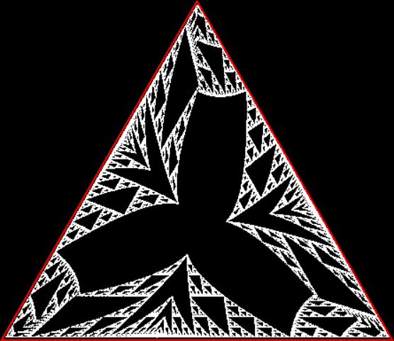
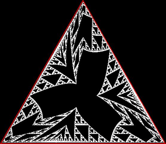
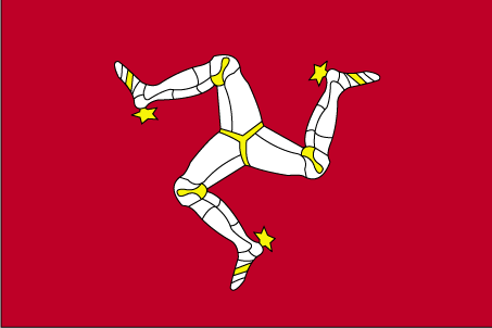
As you can see, the appearance of the Sierpiński triangle changes notably as the points rotate: the rotations aren’t rotationally symmetrical (in the standard sense). Sometimes a rotation looks like a stumpy triskelion, a three-legged shape like the flag of the Isle of Man:

Triskelion on the Manx flag (Wikipedia)


Interior points of a Sierpiński triangle rotated by 30°


But topologically speaking, each rotated triangle is the same (just as, topologically speaking, a coffee-cup is the same as a donut). You can see how they’re topologically the same by imagining that the triangle is stretched into a circle, like this:

Sierpiński triangle

↓

Sierpiński triangle stretched into circle


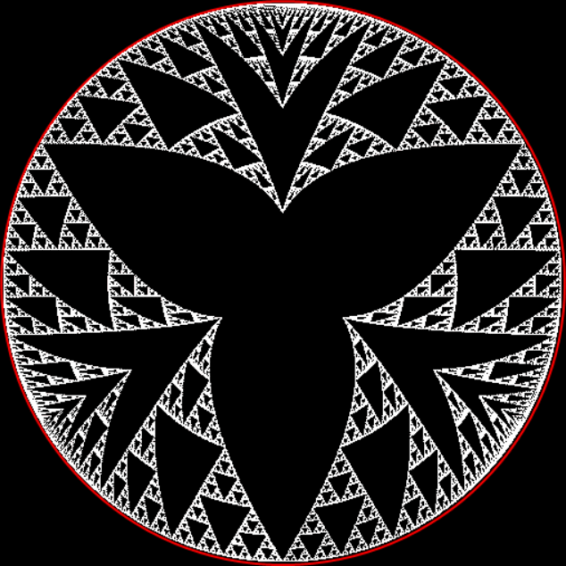
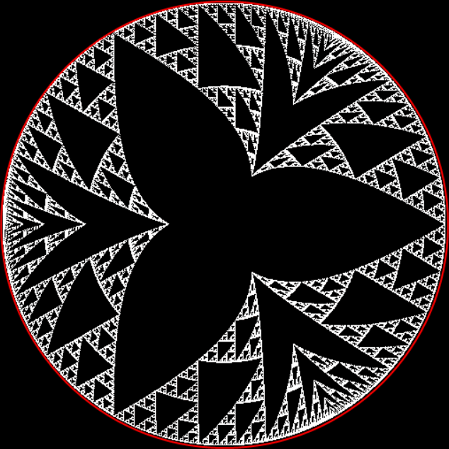
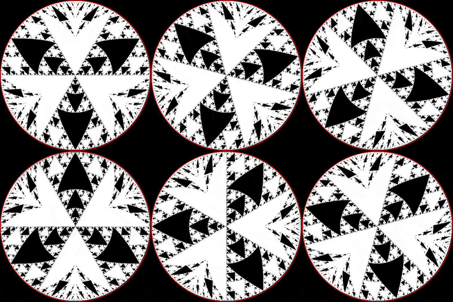
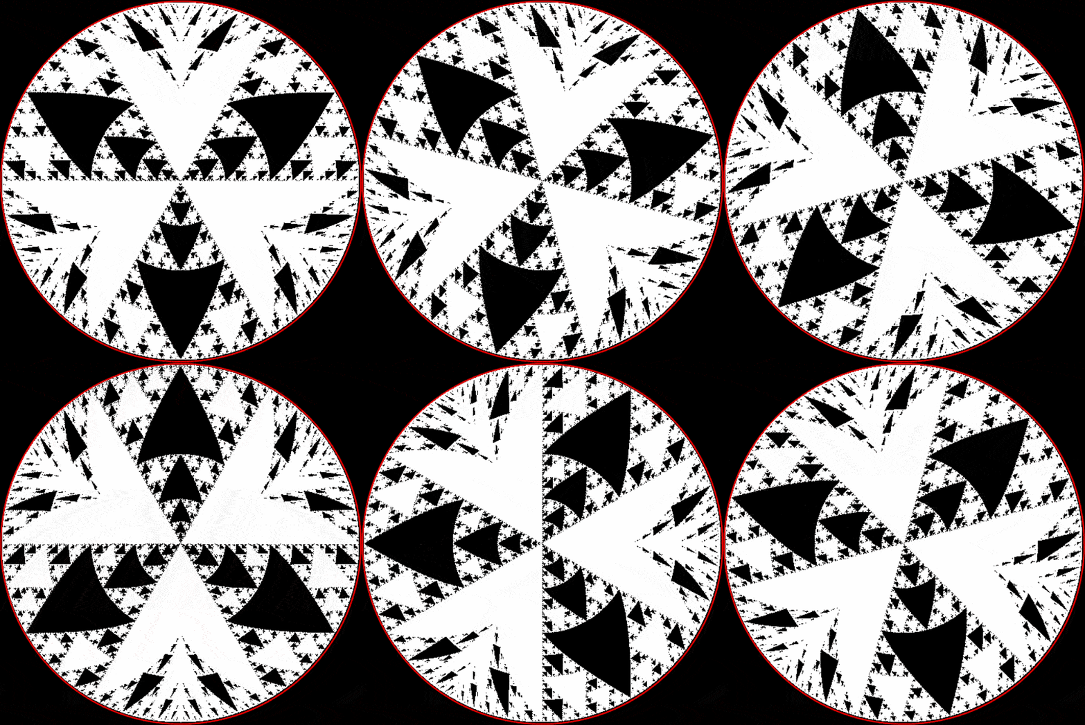
When you circularize the rotated triangles, all the circularized triangles are rotationally symmetrical:

Points rotated by 30°

↓

Circle from triangle rotated by 30°


Points rotated by 60°

↓

Circle from triangle rotated by 60°


Points rotated by 90°

↓

Circle from triangle rotated by 90°


Here are two animated gifs of the circularized triangles rotating:

Circularized Sierpiński triangle flowing around center (slow animation at ezGif)


Circularized Sierpiński triangle flowing around center (faster animation)


Here’s what I call the centered Sierpiński triangle turned into a circle:

Centered Sierpiński triangle


↓

Circle from centered Sierpiński triangle


And finally, the circularized centered Sierpiński triangle flowly rotating at two speeds:

Circularized centered Sierpiński triangle flowing around center (slow animation at ezGif)


Circularized centered Sierpiński triangle flowing around center (faster animation)


A FracTeasel on a Fract-L

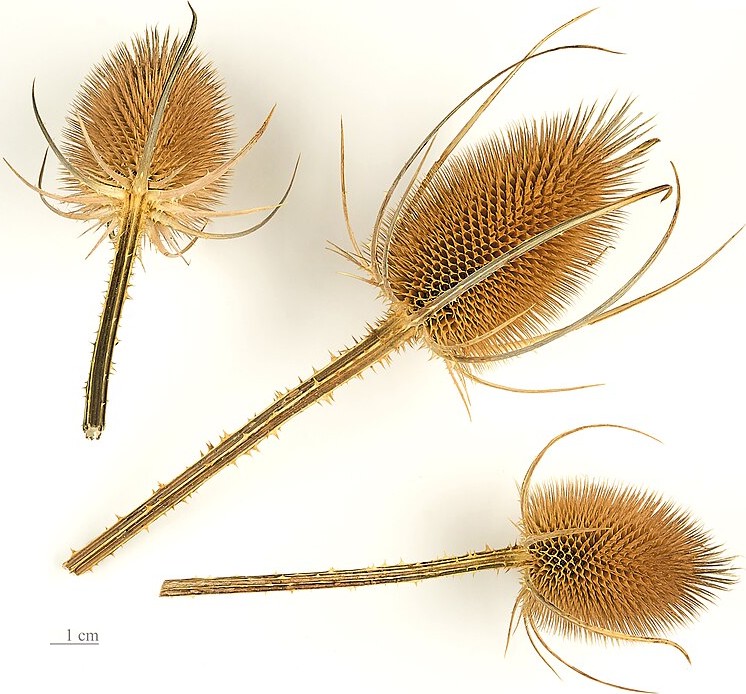
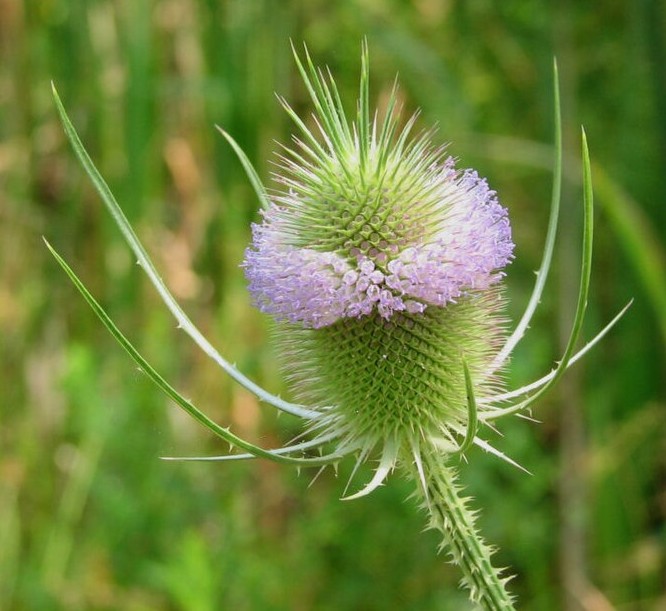
Here are two new fractals, both of which remind me of the seedheads of the wildflower known as a teasel, Dipsacus fullonum:

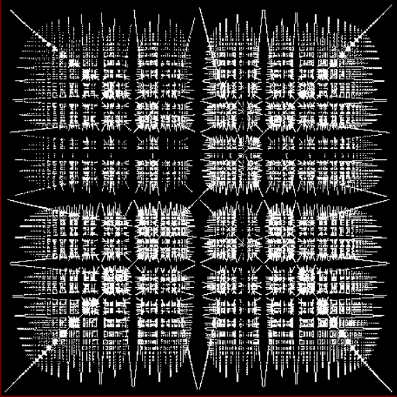
A FracTeasel fractal


Dried seedheads of teasel, Dipsacus fullonum (Wikipedia)


Another FracTeasel fractal (embedded in the first)


Flowering seedhead of teasel, Dipsacus fullonum (Wikipedia)


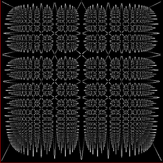
How do you create the two FracTeasels? Let’s look first at the fractal they’re inspired by. In “Back to Frac’” I talked about this fractional fractal, a variant of what I call the limestone fractal:

Variant of a limestone fractal or gryke fractal


It’s a fractal on a fract-L, that is, the x and y co-ordinates of the red L represent pairs of fractions generating decimals between 0 and 1. The x represents the fractions a1/b1 = 1/n to (n-1)/n in simplest form: 1/2, 1/3, 2/3, 1/4, 3/4, 1/5, 2/5, 3/5, 4/5, 1/6, 5/6, 1/7, 2/7, 3/7, 4/7, 5/7, 6/7, 1/8, 3/8, 5/8, 7/8,…

And what about the y? It represents the fraction found by taking the continued fraction of a1/b1, reversing it, and generating a new fraction, a2/b2, from the reversal. For example, here’s the continued fraction of a1/b1 = 3/23 = 0.1304347826…:

contfrac(3/23) = 7,1,2

The continued fraction of a1/b1 = 3/23 is used like this to reconstruct a1/b1:

7,1,2

0 → 1 / (0 + 2) = 1/2 → 1 / (1/2 + 1) = 2/3 → 1 / (7 + 2/3) = 3/23

Now reverse the continued fraction, 7,1,2 → 2,1,7, and generate a2/b2:

2,1,7

0 → 1 / (0 + 7) = 1/7 → 1 / (1/7 + 1) = 7/8 → 1 / (2 + 7/8) = 8/23 = 0.3478260869565…

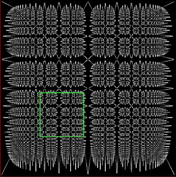
The limestone fractal above appears when a1/b1 → a2/b2 for a1/b1 = 1/2, 1/3, 2/3, 1/4, 3/4, 1/5, 2/5, 3/5, 4/5, 1/6, 5/6, 1/7, 2/7, 3/7, 4/7, 5/7, 6/7, 1/8, 3/8, 5/8, 7/8,… But you can do other things to contfrac(a1/b1) beside just reversing it. What about the permutations of contfrac(a1/b1), for example? If length(contfrac(a1/b1)) = n, the permutations can generate up to n! (factorial n) new a2/b2 for the y co-ordinate (if all the numbers of contfrac(a1/b1) are different, you’ll get n! permutations). The resultant fractal is the first of the FracTeasels above (note that a2/b2 isn’t multiplied by two):

FracTeasel #1 from fract-L for y = perm(contfrac(a1/b1))


If you think about it, you’ll see that the fractal from permed contfrac(a1/b1) contains the fractal from reversed contfrac(a1/b1). It also contains the second FracTeasel:

FracTeasel #2


How so? Because the second FracTeasel — let’s call it the stemmed FracTeasel — is created by shifting some numbers in contfrac(a1/b1) and leaving others alone. For example:

contfrac(940/1089) = 1, 6, 3, 4, 5, 2 → 1, 4, 3, 2, 5, 6 = contfrac(1008/1243)

So the function is finding one particular permutation of contfrac(a1/b1) to generate a2/b2, not all permutations. And so the function creates the stemmed FracTeasel, which carries an infinite number of seedheads on the same stem. To show that, here’s an animated gif zooming in on the bend of the fract-L for the stemmed FracTeasel:

Zooming the FracTeasel (animated at ezGif)


Elsewhere Other-Accessible…

• I Like Gryke — a first look at the limestone fractal
• Lime Time — more on the limestone fractal

Back to Frac’

Here’s a second serendipitous fractal:
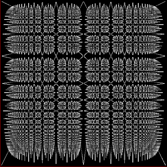
A serendipitous fractal on a fract-L


It looks like (and is related to) the limestone fractal and I found it similarly serendipitously. This time I was looking at continued fractions, a simple yet subtle and seductive way of representing non-integer numbers like 2/3 and 7/9 (or √2 and π). To generate a continued fraction from a/b < 1, you divide a/b into 1 and take away the integer part. Then you repeat with the remainder until nothing is left (or, as with irrationals like 1/√2 and 1/π, you've calculated long enough for your needs). The integers at each stage are the numbers of the continued fraction. Here is the working for contfrac(2/3), the continued fraction of 2/3:

int(1/(2/3)) = int(3/2) = int(1.5) = 1
3/2 – 1 = 1/2
int(1/(1/2)) = int(2) = 2
2 – 2 = 0

contfrac(2/3) = 1, 2

By working backwards with (1, 2), you can use the continued fraction to reconstruct the original number a/b. Start with a/b = 0/1:

1 / (0/1 + 2) = 1 / ((0+2*1)/2) = 1 / (2/1) = 1/2
1 / (1/2 + 1) = 1 / ((1+2*1)/2) = 1 / (3/2) = 2/3

And here’s the working for contfrac(7/9), the continued fraction of 7/9:

int(1/(7/9)) = int(9/7) = int(1.285714…) = 1
9/7 – 1 = 2/7
int(1/(2/7)) = int(7/2) = int(3.5) = 3
7/2 – 3 = 1/2
int(1/(1/2)) = int(2) = 2
2 – 2 = 0

contfrac(7/9) = 1, 3, 2

And here’s the reconstruction of 7/9 from its continued fraction, starting again with a/b = 0/1:

1 / (0/1 + 2) = 1 / ((0+2*1)/2) = 1 / (2/1) = 1/2
1 / (1/2 + 3) = 1 / ((1+2*3)/2) = 1 / (7/2) = 2/7
1 / (2/7 + 1) = 1 / ((2+7*1)/7) = 1 / (9/7) = 7/9

From that simple algorithm arise subtle and seductive things. Look at some continued fractions, cf(a/b), for a/b in simplest form (giving only the first few reciprocals, 1/b, because cf(1/b) = b). Interesting patterns appear, e.g. when a/b uses adjacent or nearly adjacent Fibonacci numbers:

cf(1/3) = 3 = cf(0.333333333…)
cf(2/3) = 1,2 = cf(0.666666666…)
cf(1/4) = 4 = cf(0.25)
cf(3/4) = 1,3 = cf(0.75)
cf(1/5) = 5 = cf(0.2)
cf(2/5) = 2,2 = cf(0.4)
cf(3/5) = 1,1,2 = cf(0.6)
cf(4/5) = 1,4 = cf(0.8)
cf(5/6) = 1,5 = cf(0.833333333…)
cf(2/7) = 3,2 = cf(0.285714285…)
cf(3/7) = 2,3 = cf(0.428571428…)
cf(4/7) = 1,1,3 = cf(0.571428571…)
cf(5/7) = 1,2,2 = cf(0.714285714…)
cf(6/7) = 1,6 = cf(0.857142857…)
cf(3/8) = 2,1,2 = cf(0.375)
cf(5/8) = 1,1,1,2 = cf(0.625)
cf(7/8) = 1,7 = cf(0.875)
cf(2/9) = 4,2 = cf(0.222222222…)
cf(4/9) = 2,4 = cf(0.444444444…)
cf(5/9) = 1,1,4 = cf(0.555555555…)
cf(7/9) = 1,3,2 = cf(0.777777777…)
cf(8/9) = 1,8 = cf(0.888888888…)
cf(3/10) = 3,3 = cf(0.3)
cf(7/10) = 1,2,3 = cf(0.7)
cf(9/10) = 1,9 = cf(0.9)
cf(2/11) = 5,2 = cf(0.181818181…)
cf(3/11) = 3,1,2 = cf(0.272727272…)
cf(4/11) = 2,1,3 = cf(0.363636363…)
cf(5/11) = 2,5 = cf(0.454545454…)
cf(6/11) = 1,1,5 = cf(0.545454545…)
cf(7/11) = 1,1,1,3 = cf(0.636363636…)
cf(8/11) = 1,2,1,2 = cf(0.727272727…)
cf(9/11) = 1,4,2 = cf(0.818181818…)
cf(10/11) = 1,10 = cf(0.909090909…)
cf(5/12) = 2,2,2 = cf(0.416666666…)
cf(7/12) = 1,1,2,2 = cf(0.583333333…)
cf(11/12) = 1,11 = cf(0.916666666…)
cf(2/13) = 6,2 = cf(0.153846153…)
cf(3/13) = 4,3 = cf(0.230769230…)
cf(4/13) = 3,4 = cf(0.307692307…)
cf(5/13) = 2,1,1,2 = cf(0.384615384…)
cf(6/13) = 2,6 = cf(0.461538461…)
cf(7/13) = 1,1,6 = cf(0.538461538…)
cf(8/13) = 1,1,1,1,2 = cf(0.615384615…)
cf(9/13) = 1,2,4 = cf(0.692307692…)
cf(10/13) = 1,3,3 = cf(0.769230769…)
cf(11/13) = 1,5,2 = cf(0.846153846…)
cf(12/13) = 1,12 = cf(0.923076923…)
cf(3/14) = 4,1,2 = cf(0.214285714…)
cf(5/14) = 2,1,4 = cf(0.357142857…)
cf(9/14) = 1,1,1,4 = cf(0.642857142…)
cf(11/14) = 1,3,1,2 = cf(0.785714285…)
cf(13/14) = 1,13 = cf(0.928571428…)
cf(2/15) = 7,2 = cf(0.133333333…)
cf(4/15) = 3,1,3 = cf(0.266666666…)
cf(7/15) = 2,7 = cf(0.466666666…)
cf(8/15) = 1,1,7 = cf(0.533333333…)
cf(11/15) = 1,2,1,3 = cf(0.733333333…)
cf(13/15) = 1,6,2 = cf(0.866666666…)
cf(14/15) = 1,14 = cf(0.933333333…)
cf(3/16) = 5,3 = cf(0.1875)
cf(5/16) = 3,5 = cf(0.3125)
cf(7/16) = 2,3,2 = cf(0.4375)

After investigating some of those patterns, I wondered what happened when you reversed the continued fraction cf(a/b) and used those reversed numbers backward (that is, used the numbers of cf(a/b) forward) to generate another and different a/b. And a/b will always be different unless cf(a/b) is a palindrome, like cf(5/12) = 2,2,2 or cf(5/13) = 2,1,1,2 or cf(4/15) = 3,1,3. Note that a continued fraction never ends in 1, so that when reversing, say, cf(5/8) = (1, 1, 1, 2), you need an adjustment from (2, 1, 1, 1) to (2, 1, 1+1) = (2, 1, 2). Here’s a little of what happens when you reverse cf(a1/b1) to generate a2/b2:

cf(1/2) = 2 → 2 = cf(1/2)
1/2 = 0.5 : 0.5 = 1/2
cf(1/3) = 3 → 3 = cf(1/3)
1/3 = 0.333333333 : 0.333333333 = 1/3
cf(2/3) = 1, 2 → 2, 1 → 3 = cf(1/3)
2/3 = 0.666666666 : 0.333333333 = 1/3
cf(3/4) = 1, 3 → 3, 1 → 4 = cf(1/4)
3/4 = 0.75 : 0.25 = 1/4
cf(2/5) = 2, 2 → 2, 2 = cf(2/5)
2/5 = 0.4 : 0.4 = 2/5
cf(3/5) = 1, 1, 2 → 2, 1, 1 → 2, 2 = cf(2/5)
3/5 = 0.6 : 0.4 = 2/5
cf(4/5) = 1, 4 → 4, 1 → 5 = cf(1/5)
4/5 = 0.8 : 0.2 = 1/5
cf(5/6) = 1, 5 → 5, 1 → 6 = cf(1/6)
5/6 = 0.833333333 : 0.166666666 = 1/6
cf(2/7) = 3, 2 → 2, 3 = cf(3/7)
2/7 = 0.285714286 : 0.428571428 = 3/7
cf(3/7) = 2, 3 → 3, 2 = cf(2/7)
3/7 = 0.428571429 : 0.285714286 = 2/7
cf(4/7) = 1, 1, 3 → 3, 1, 1 → 3, 2 = cf(2/7)
4/7 = 0.571428571 : 0.285714286 = 2/7
cf(5/7) = 1, 2, 2 → 2, 2, 1 → 2, 3 = cf(3/7)
5/7 = 0.714285714 : 0.428571429 = 3/7
cf(6/7) = 1, 6 → 6, 1 → 7 = cf(1/7)
6/7 = 0.857142857 : 0.142857143 = 1/7
cf(3/8) = 2, 1, 2 → 2, 1, 2 = cf(3/8)
0.375 : 0.375
cf(5/8) = 1, 1, 1, 2 → 2, 1, 1, 1 → 2, 1, 2 = cf(3/8)
0.625 : 0.375
cf(7/8) = 1, 7 → 7, 1 → 8 = cf(1/8)
0.875 : 0.125
cf(2/9) = 4, 2 → 2, 4 = cf(4/9)
0.222222222 : 0.444444444
cf(4/9) = 2, 4 → 4, 2 = cf(2/9)
0.444444444 : 0.222222222

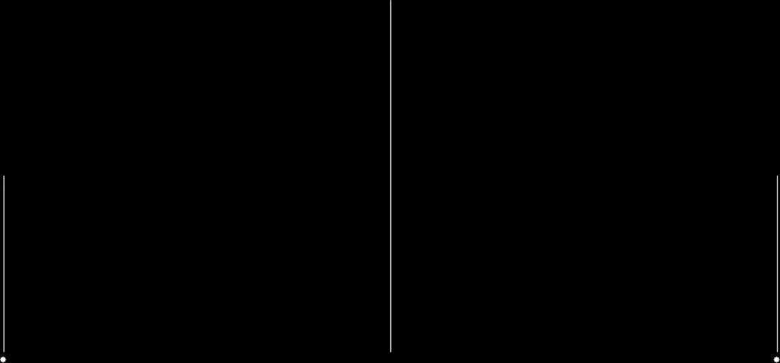
And if you plot x = a1/b1 and y = (a2/b2 * 2) on a fract-L, that is, a graph whose horizontal and vertical arms represent 0 to 1, you get the fractal right at the beginning:

Fract-L for x = a1/b1 and y = (a2/b2 * 2), where a2/b2 is generated from reversed(cf(a1/b1))


You need to use (a2/b2 * 2) because a2/b2 from reversed(cf(a1/b1)) is always <= 0.5, so using raw a2/b2 generates this graph:
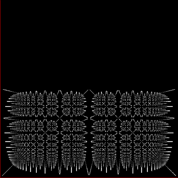
Fract-L for x = a1/b1 and y = a2/b2 (i.e. a2/b2 is unadjusted)


Why is it always true that a2/b2 <= 0.5? For two reasons. First, a/b > 0.5 always generate continued fractions that start with 1, like cf(2/3) = 1, 2 or cf(3/4) = 1, 3 or cf(3/5) = 1, 1, 2. Second, as previously mentioned, no continued fraction ends with 1. Therefore a reversed cf(a1/b1), where the final number, n > 1, moves to the beginning, will never begin with 1 and the a2/b2 generated from reversed(cf(a1/b1)) will always be less than 0.5 (or equal to it in the solitary case of cf(1/2) = 2).

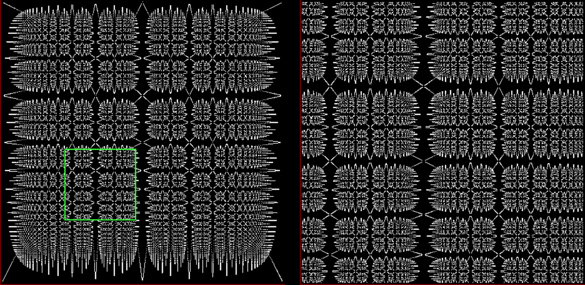
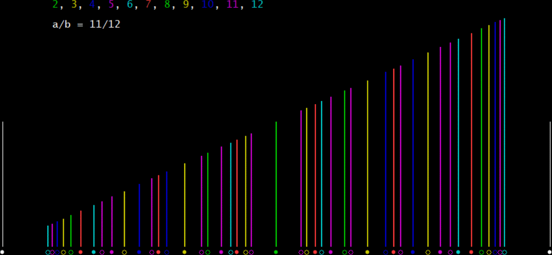
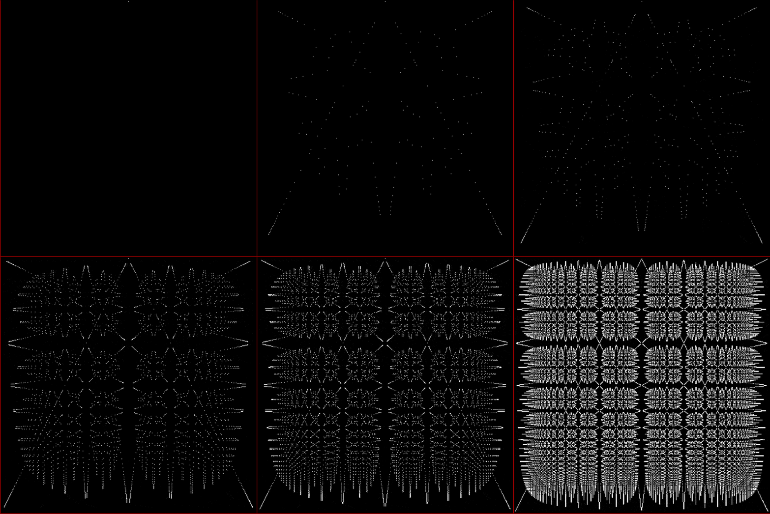
Now let's look at the development of the fractal as a1/b1 uses larger and larger denominators:
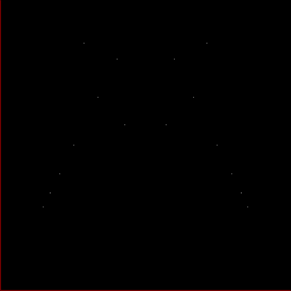
Fract-L for x = a1/b1 and y = (a2/b2 * 2) for a1/b1 <= 6/7
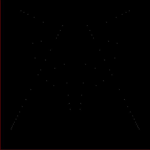

Fract-L for for a1/b1 <= 14/15
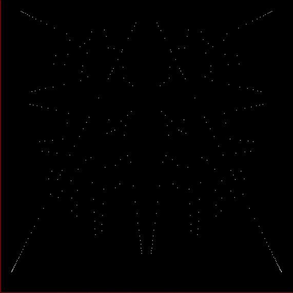

Fract-L for a1/b1 <= 30/31
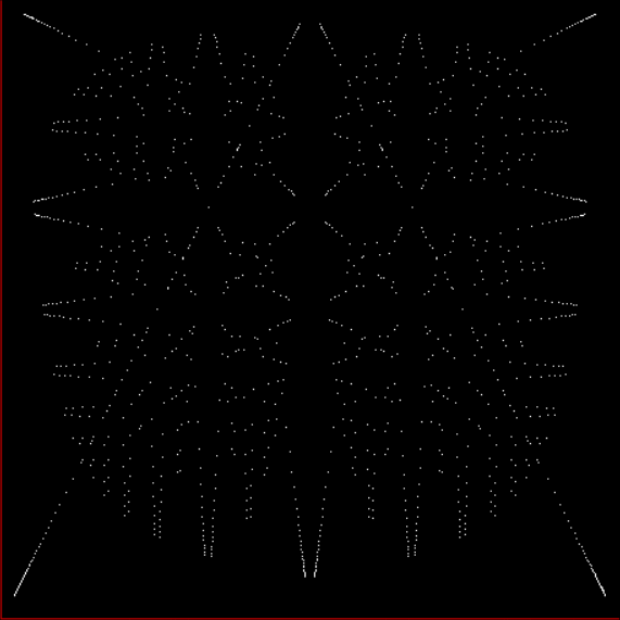

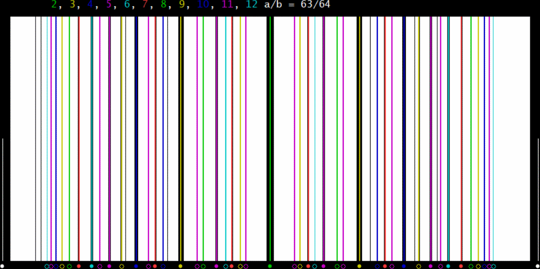
Fract-L for a1/b1 <= 62/63
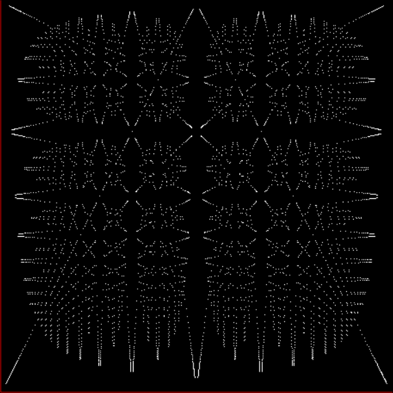

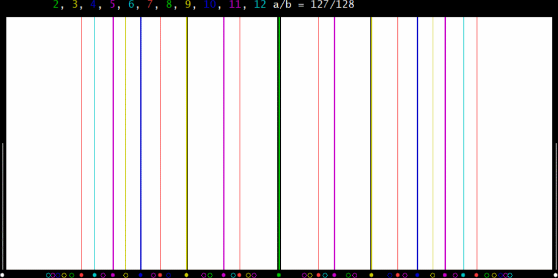
Fract-L for a1/b1 <= 126/127
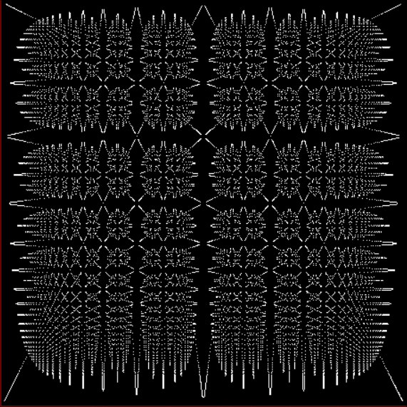

Fract-L for a1/b1 <= 254/255
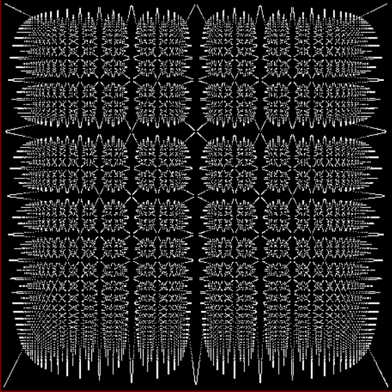

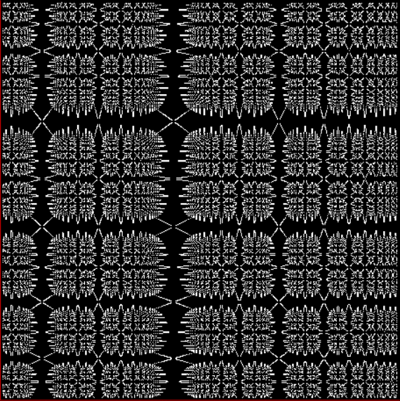
Fract-L for a1/b1 <= 357/358


Fract-L for a1/b1 <= 467/468
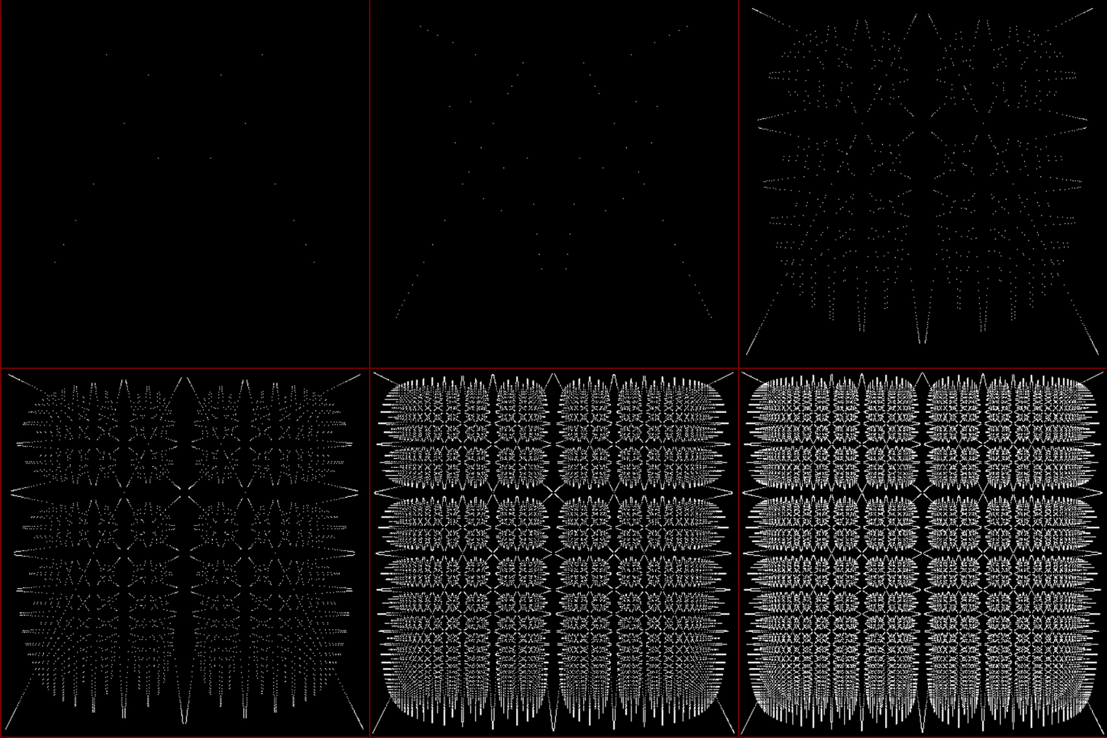

Animated fract-L for x = a1/b1 and y = (a2/b2 * 2) (animated at ezGif)


The fractal changes subtly when you restrict the b1 of a1/b1 in some way, say using multiples of 2, 3, 4, 5…:
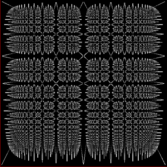
Fract-L for x = a1/b1 and y = (a2/b2 * 2) for b1 = n = 2, 3, 4, 5, 6, 7, 8…
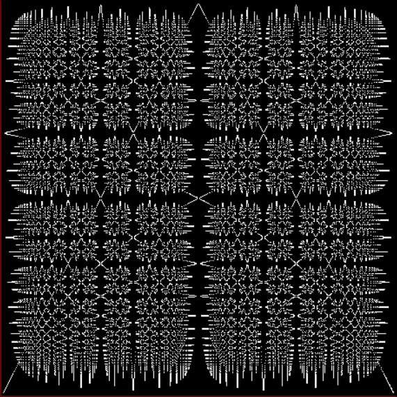

Fract-L for b1 = 2n = 2, 4, 6, 8, 10…
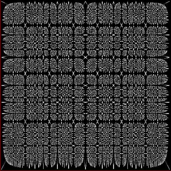

Fract-L for b1 = 3n = 3, 6, 9, 12, 15…
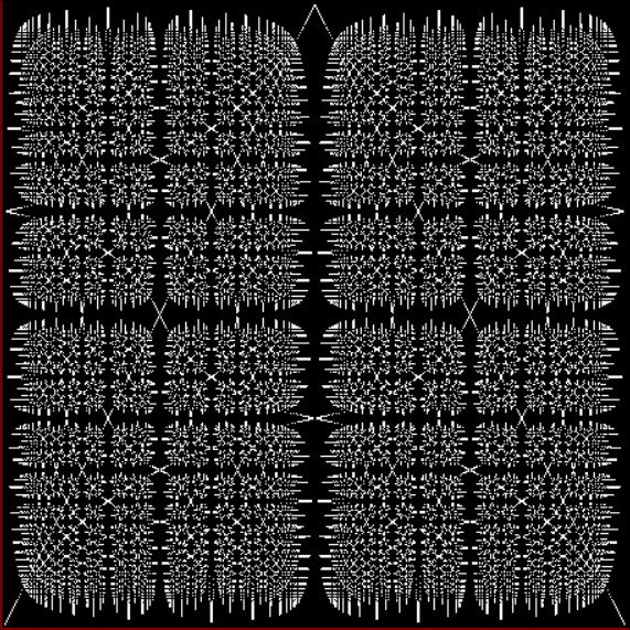

Fract-L for b1 = 4n
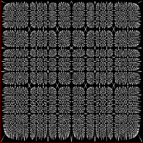

Fract-L for b1 = 5n
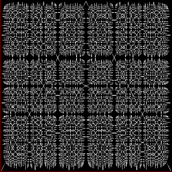

Fract-L for b1 = 6n
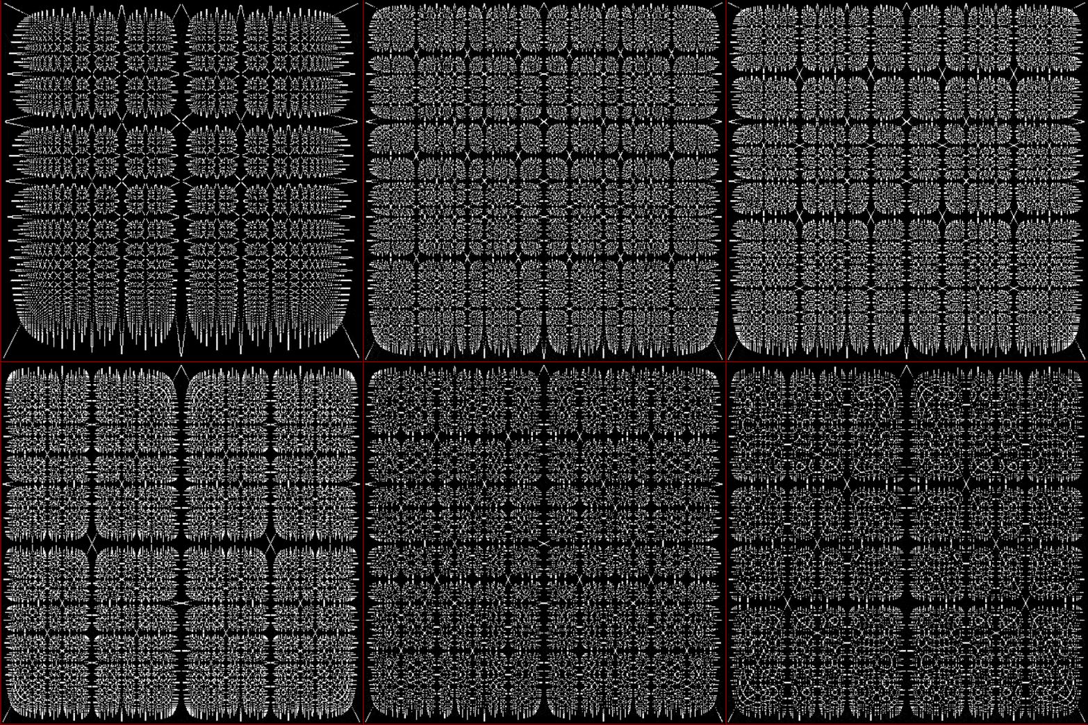

Animated fract-L for b1 = 1n..12n (animated at ezGif)


Finally, here are fract-Ls when b1 is a triangular, square, hexagonal or octagonal number:
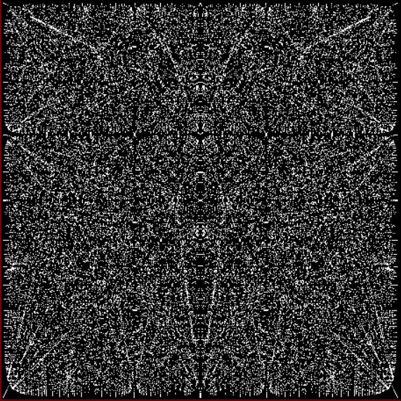
Fract-L for x = a1/b1 and y = (a2/b2 * 2) for triangular(b1) = 3, 6, 10, 15, 21, 28,…
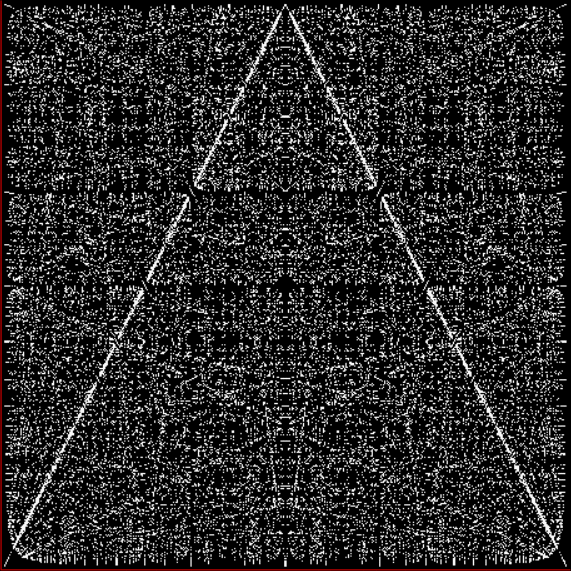

Fract-L for square(b1) = 4, 9, 16, 25, 36, 49,…
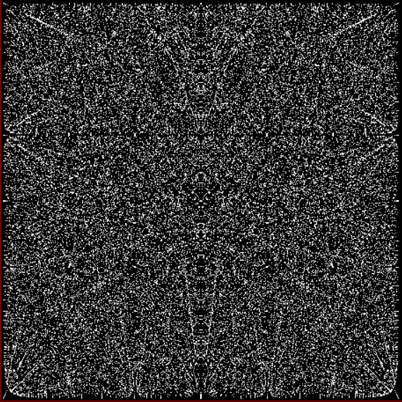

Fract-L for hexagonal(b1) = 6, 15, 28, 45, 66, 91,…
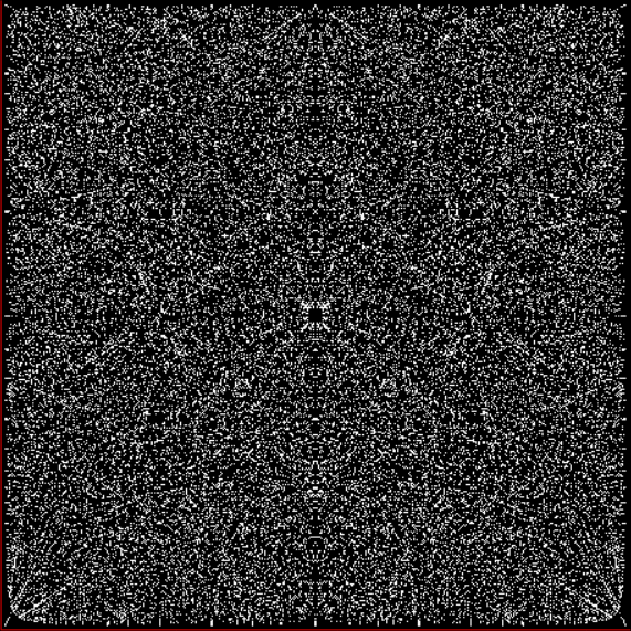

Fract-L for octagonal(b1) = 8, 21, 40, 65, 96, 133,…


Elsewhere Other-Accessible…

• Back to Drac’ — a parallel pun for a pre-previous fractal
• I Like Gryke — a first look at the limestone fractal
• Lime Time — more on the limestone fractal

Fractional Fractal Fract-Ls

This is the surpassingly special Stern-Brocot sequence:

0, 1, 1, 2, 1, 3, 2, 3, 1, 4, 3, 5, 2, 5, 3, 4, 1, 5, 4, 7, 3, 8, 5, 7, 2, 7, 5, 8, 3, 7, 4, 5, 1, 6, 5, 9, 4, 11, 7, 10, 3, 11, 8, 13, 5, 12, 7, 9, 2, 9, 7, 12, 5, 13, 8, 11, 3, 10, 7, 11, 4, 9, 5, 6, 1, 7, 6, 11, 5, 14, 9, 13, 4, 15, 11, 18, 7, 17, 10, 13, 3, 14, 11, 19, 8, 21, 13, 18, 5, 17, 12, 19, … (A002487 at the Online Encyclopedia of Integer Sequences)


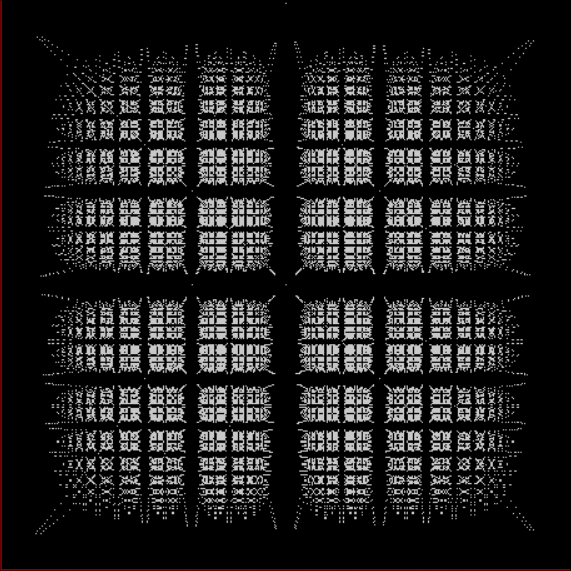
And why is the sequence special? Because if you take successive pairs of the apparently arbitrarily varying numbers, you get every rational fraction in its simplest form exactly once. So 1/2, 2/3, 6/11 and 502/787 appear once and then never again. And so do 2/1, 3/2, 11/6 and 787/502. Et cetera, ad infinitum. If you map the Stern-Brocot sequence against the related Calkin-Wilk sequence, which has the same “all-simplest-fractions-exactly-once” properties, you can create this fractal, which I call a limestone fractal or gryke fractal:

Gryke fractal by mapping Stern-Brocot sequence against Calkin-Wilf sequence


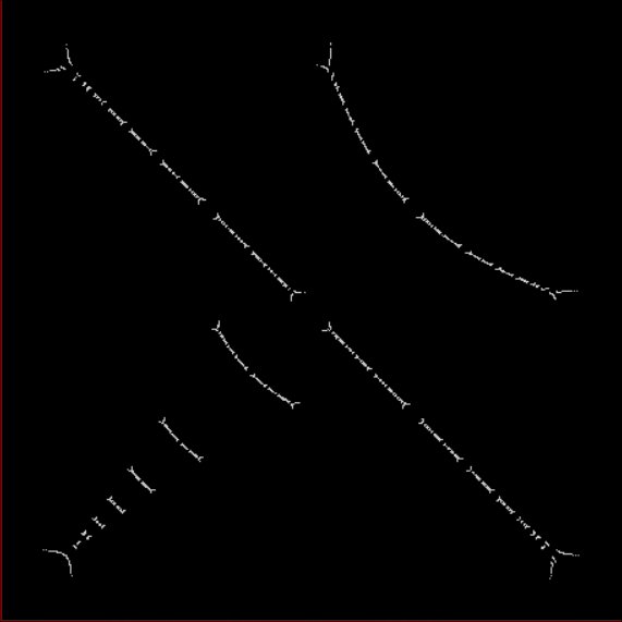
The graph is what I call a Fract-L, because the lines for the x,y coordinates create an L. Each coordinate runs from 0 to 1, with the x set by the fraction from the Stern-Brocot sequence and the y set by the fraction from the Calkin-Wilf sequence (if a > b in a/b, use the conversion 1/(a/b) = b/a). But you can also find interesting patterns by mapping the Stern-Brocot sequence against itself. That is, you use two Stern-Brocot sequences that start in different places. Now, there are complicated ways to create the Stern-Brocot sequence using mathematical trees and sequential algorithms and so on. But there’s also an astonishingly simple way, a formula created by the Israeli mathematician Moshe Newman. If (a,b) is one pair of successive numbers in the sequence, the next pair (a,b) is found like this:

c = b
b = (2 * int(a/b) + 1) * b – a
a = c

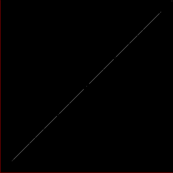
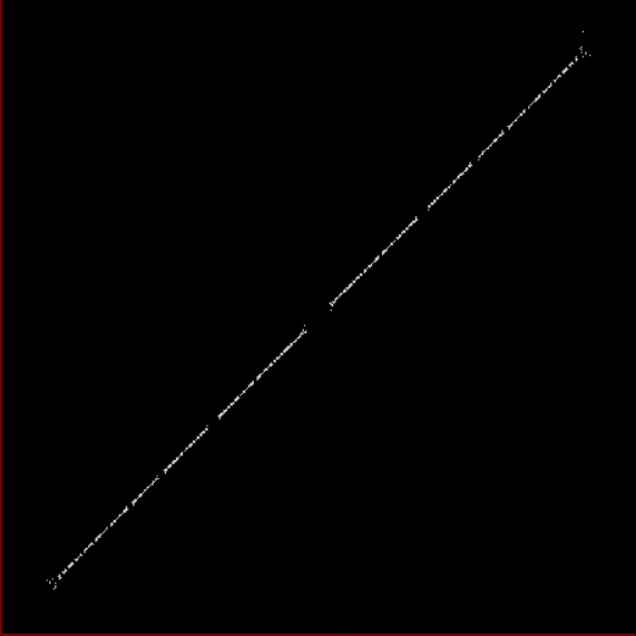
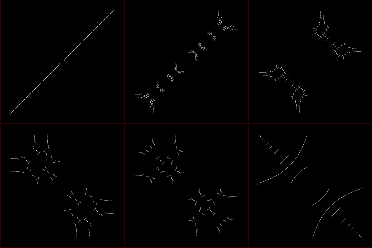
This means that you can seed a Stern-Brocot sequence with any (correctly simplified) a/b and it will continue in the right way. If the two SB-sequences for x and y are both seeded with (0,1), you get this 45° line, because each successive a/b for (x,y) is identical:

Stern-Brocot pairs seeded with x ← (0,1) and y ← (0,1)


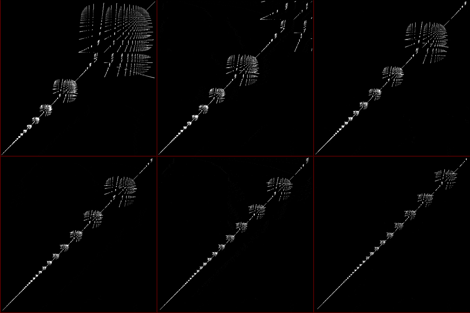
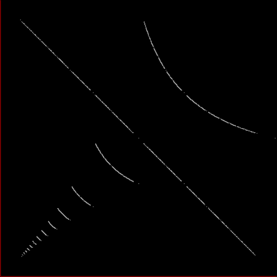
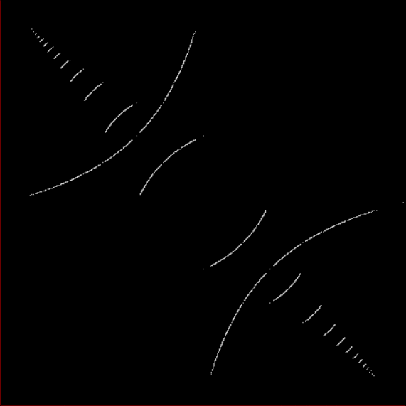
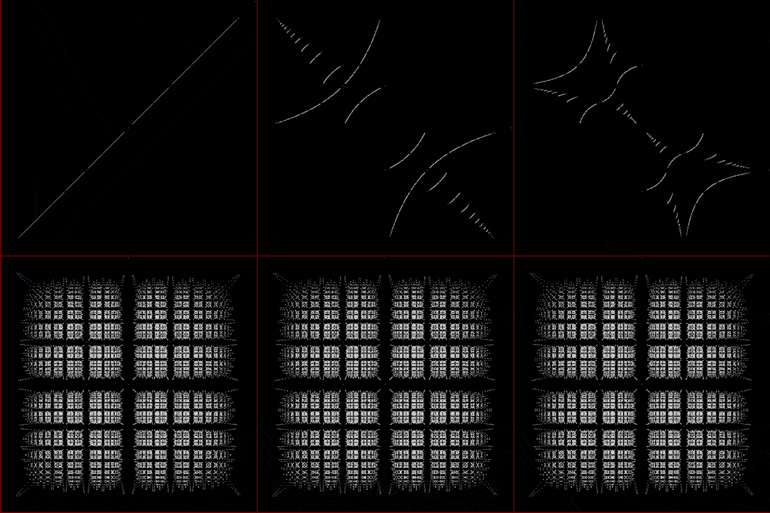
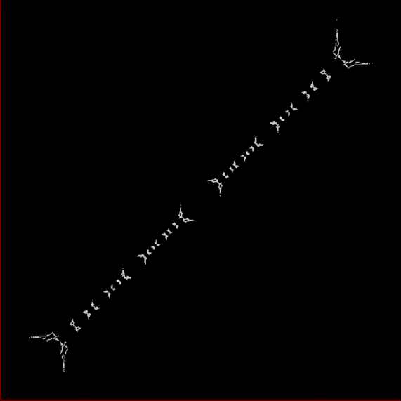
The further you extend the sequences, the less broken the 45° line will appear, because the points determined by a/b for x and y will get closer and closer together (but the line will never be solid, because any two rationals are separated by an infinity of irrationals). Now try offsetting the SB-sequences for x,y by using different seeds. Different fractal patterns appear, which all appear to be subsets (or fractions) of the limestone fractal above (see animated gif below):
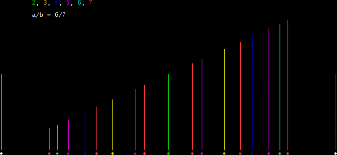
Stern-Brocot pairs seeded with x ← (0,1) and y ← (1,1)


x ← (0,1) and y ← (1,2)


x ← (0,1) and y ← (1,3)


x ← (0,1) and y ← (2,3)


x ← (0,1) and y ← (3,4)


x ← (0,1) and y ← (6,7)


x ← (1,2) and y ← (1,9)


x ← (1,4) and y ← (1,6)


x ← (1,7) and y ← (1,8)


x ← (2,3) and y ← (4,5) — apparently identical to x ← (1,4) and y ← (1,6) above


x ← (26,25) and y ← (1,10)


Gryke fractal compared with Stern-Brocot-pair patterns (animated at ezGif)


And here’s what happens when the seed-fractions for x run from 1/3 to 12/13, while the seed-fraction for y is held constant at 1/23:

x ← (1,13) and y ← (1,23)


x ← (2,13) and y ← (1,23)


x ← (3,13) and y ← (1,23)


x ← (4,13) and y ← (1,23)


x ← (5,13) and y ← (1,23)


x ← (6,13) and y ← (1,23)


x ← (7,13) and y ← (1,23)


x ← (8,13) and y ← (1,23)


x ← (9,13) and y ← (1,23)


x ← (10,13) and y ← (1,23)


x ← (11,13) and y ← (1,23)


x ← (12,13) and y ← (1,23)


Animated gif for x ← (n,13) and y ← (1,23) (animated at ezGif)


Previously Pre-Posted

• I Like Gryke — a first look at the limestone fractal
• Lime Time — more on the fractal
The Wyrm Ferns

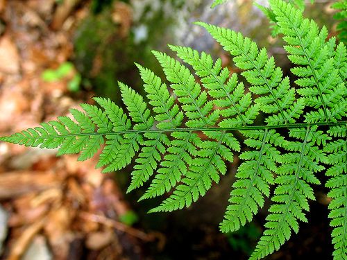
A fern is a fractal, a shape that contains copies of itself at smaller and smaller scales. That is, part of a fern looks like the fern as a whole:

Fern as fractal (source)

Millions of years after Mother Nature, man got in on the fract, as it were:

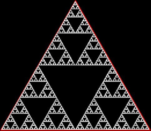
The Sierpiński triangle, a 2d fractal

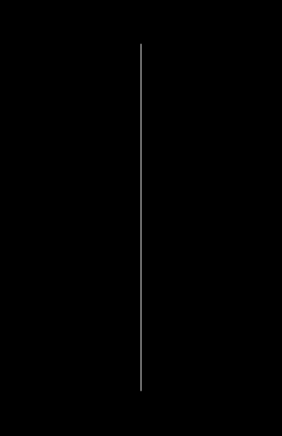
The Sierpiński triangle is a fractal created in two dimensions by a point jumping halfway towards one or another of the three vertices of a triangle. And here is a fractal created in one dimension by a point jumping halfway towards one or another of the two ends of a line:
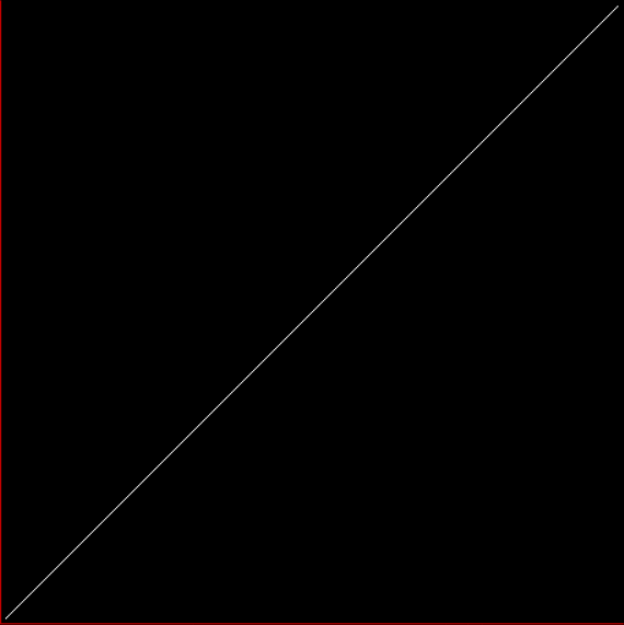
A 1d fractal

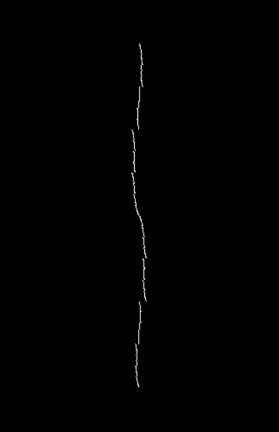
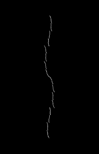
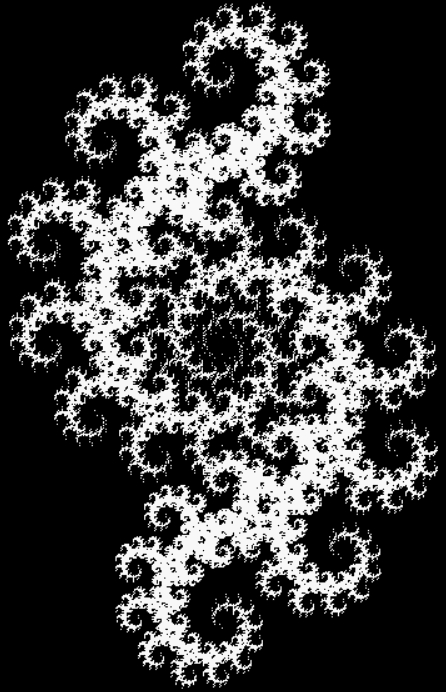
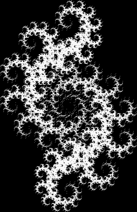
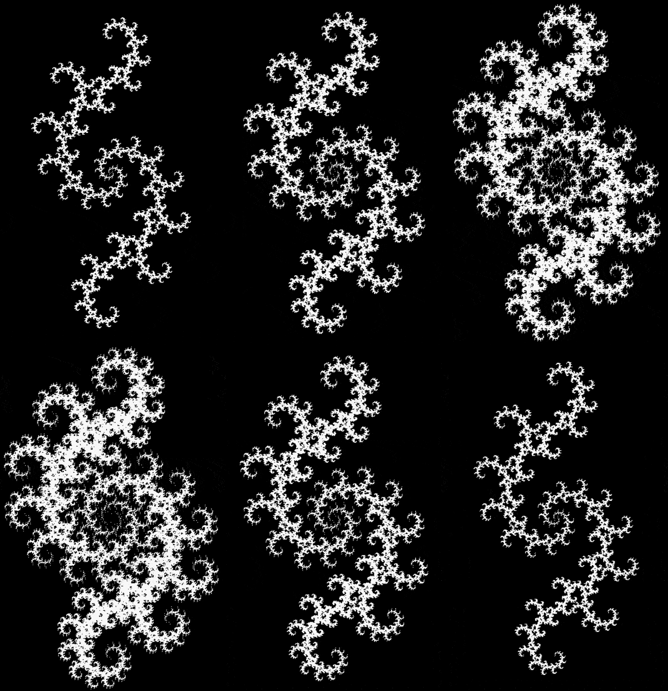
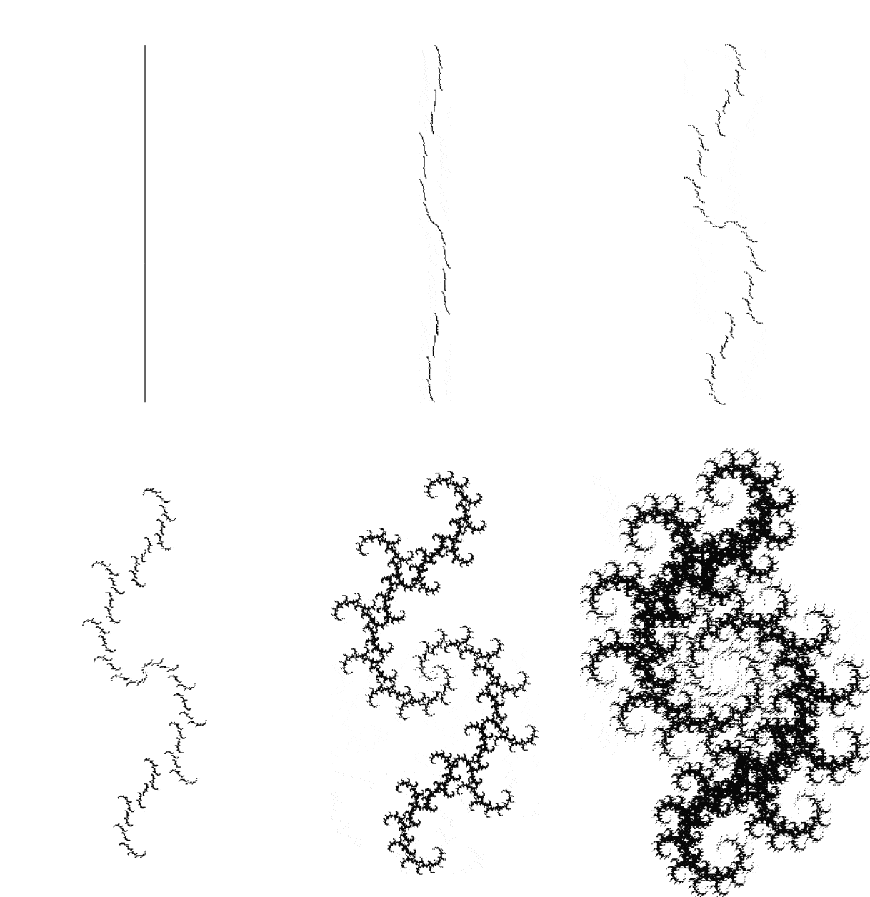
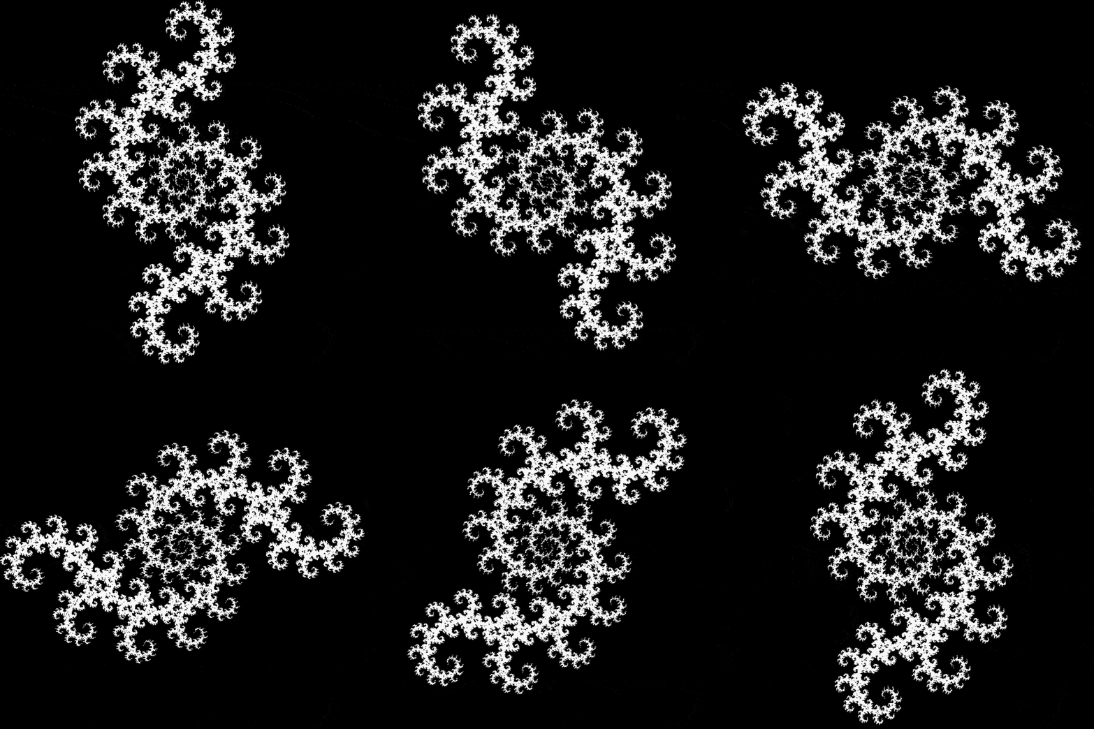
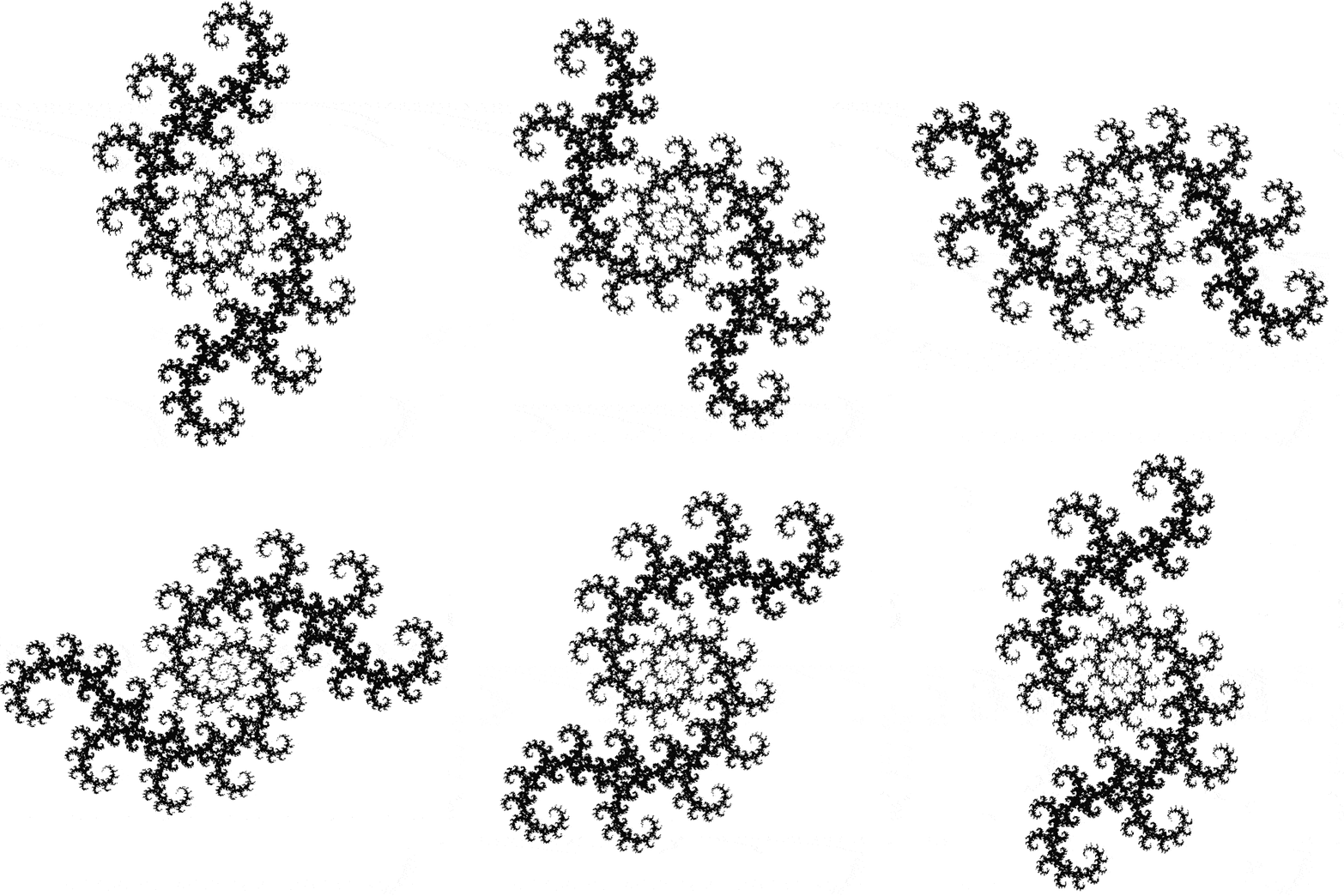
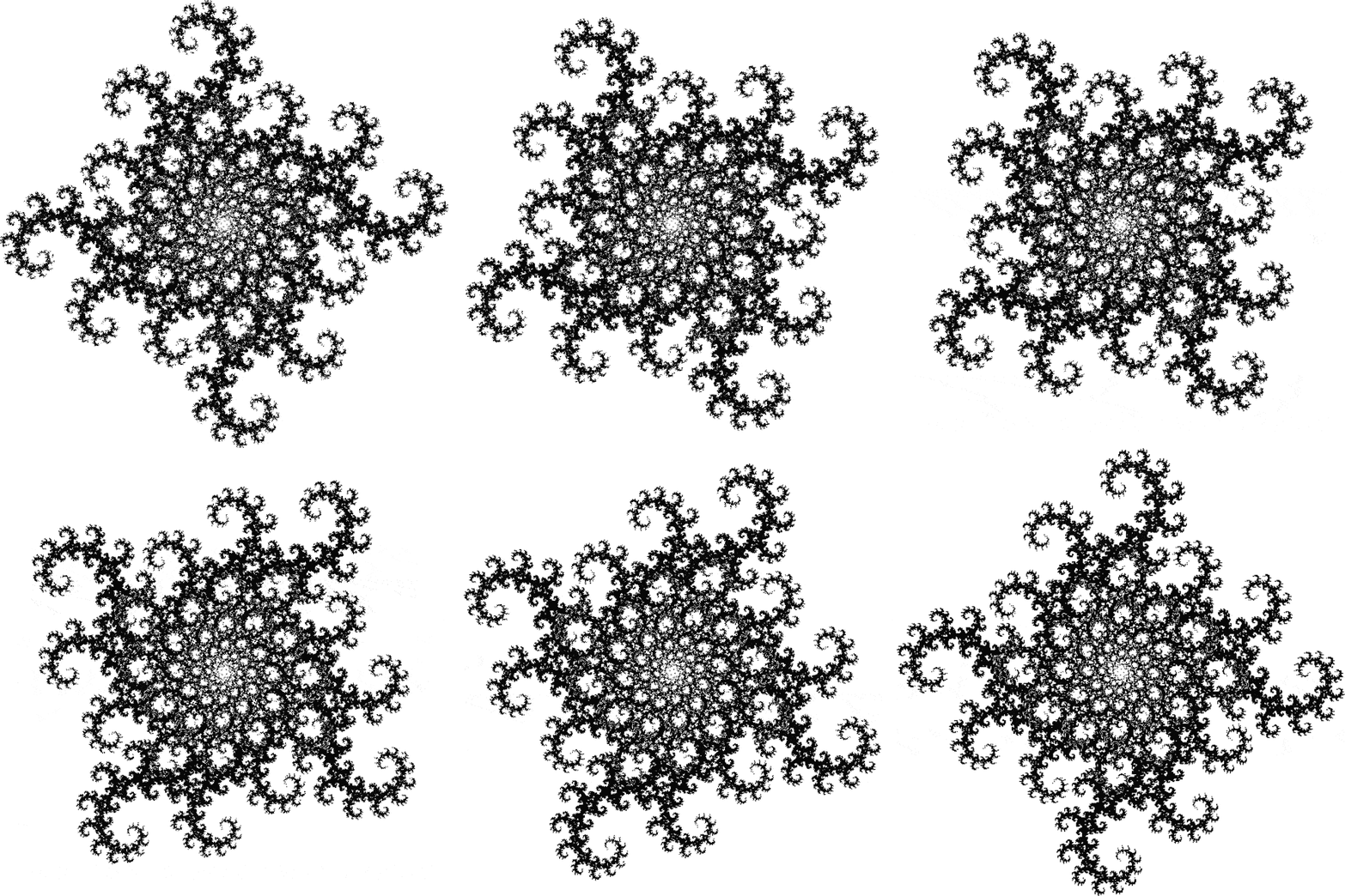
In one dimension, the fractality of the fractal isn’t obvious. But you can try draggin’ out (or dragon out) the fractality of the fractal by ferning the wyrm, as it were. Suppose that after the point jumps halfway towards one or another of the two points, it’s rotated by some angle around the midpoint of the two original points. When you do that, the fractal becomes more and more obvious. In fact, it becomes what’s called a dragon curve (in Old English, “dragon” was wyrm or worm):
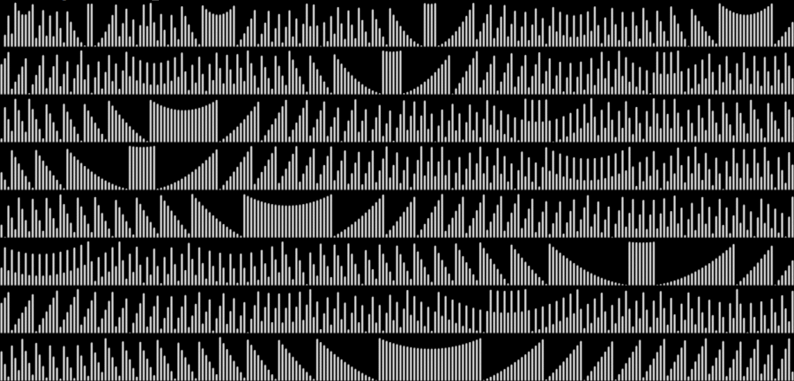
Fractal with angle = 5°


Fractal 10°


Fractal 15°


Fractal 20°


Fractal 25°


Fractal 30°


Fractal 35°


Fractal 40°


Fractal 45°


Fractal 50°


Fractal 55°


Fractal 60°


Fractal 0° to 60° (animated at ezGif)


But as the angle gets bigger, an interesting aesthetic question arises. When is the ferned wyrm, the dragon curve, at its most attractive? I’d say it’s when angle ≈ 55°:

Fractal 50°


Fractal 51°


Fractal 52°


Fractal 53°


Fractal 54°


Fractal 55°


Fractal 56°


Fractal 57°


Fractal 58°


Fractal 59°


Fractal 60°


Fractal 50° to 60° (animated)


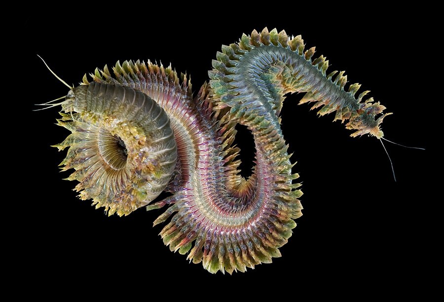
At angle >= 57°, I think the dragon curve starts to look like some species of bristleworm, which are interesting but unattractive marine worms:

A bristleworm, Nereis virens (see polychaete at Wikipedia)


Finally, here’s what the ferned wyrm looks like in black-and-white and when it’s rotating:

Fractal 0° to 60° (b&w, animated)


Fractal 56° (rotating)


Fractal 56° (b&w, rotating)


Double fractal 56° (b&w, rotating)

Previously Pre-Posted (Please Peruse)…

• Curvous Energy — a first look at dragon curves
• Back to Drac’ — another look at dragon curves

Scout the Routes

Triangles? Yes. Squares? No. If you scout the routes with a triangle, you get a beautiful fractal. If you scout the routes with a square, you don’t. Here’s what you get with a triangle:

A Sierpiński triangle


But how do you scout the routes? (That phrase works best in the American dialects where “scout” rhymes with “route”.) Simple: you mark the final positions reached when a point traces all possible ways of jumping, say, eight times 1/2-way towards the vertices of a polygon. Here’s an animation of a point scouting the routes of eight jumps towards the vertices of a triangle (it starts each time at the center):

Creating a Sierpiński triangle by scouting the routes (animated at Ezgif)


If you scout the routes with a square, you don’t get a fractal. Instead, the interior of the square fills evenly (and boringly) with the end-points of the routes:

Scouting the routes with a square (animated at Ezgif)


But you can create fractals with a square if you out routes as you scout routes. That is, if you exclude some routes and don’t mark their end-points. One way to do this is to compare the proposed next jump-vertex (vertex-jumped-towards) with the previous jump-vertex. For example, if the proposed jump-vertex, jv[t], is the same as the previous jump-vertex, jv[t-1], you don’t jump towards jv[t] or you jump towards it in a different way. The test is jv[t] = jv[t-1] + vi. If vi = 0 and you jump towards the clockwise neighbor of jv when the test is true, you get a fractal looking like this:
vi = 0, action = jv → jv + 1


Here’s the fractal if you jump towards the clockwise-neighbor-but-one when the test is true:
vi = 0, action = jv + 2


Now try varying the vi of the jv[t-1] + vi:

vi = 2, action = jv + 2


vi = 2, action = jv + 1


vi = 3, action = jv + 1


Or what about jumping in a different way towards jv when the test is true? If you jump 2/3 of the way rather 1/2, you get his fractal:

vi = 2, action = jump 2/3


And if you jump 4/3 of the way (i.e., you overshoot the vertex jv), you get this fractal:

vi = 0, action = jump 4/3rds to vertex


vi = 0, jump 4/3 (guide-square removed)


vi = 2, jump 4/3rds (guide-square removed)


And in this fractal the point jumps 2/3 of the way to the center of the square when the test is true:
vi = 2, action = jump 2/3rds of way to center of square


But why apply only one test to jv[1] and use only when one alternative jump? If jv[t] = jv[t-1] + 1 or jv[t] = jv[t-1] + 3, jv[t] becomes jv[t]+1 or jv[t]+3, respectively, you get this fractal:

vi = 1, jv + 1; vi = 3, jv + 3


Here are more fractals created by single and double tests:

vi = 1, jv + 1


vi = 0, jump 2/3


vi = 0, jump towards center 2/3rds


vi = 1, jump-center 2/3


vi = 2, jump 1/3; vi = 3, jump 1/1 (i.e, 1)


vi = 0, jv + 2; vi = 2, jump-center 1/2


vi = 0, jv + 2; vi = 2, jump-center 2/3


vi = 0, jv + 2; vi = 2, jump-center 4/3


vi = 0, jv + 1; vi = 2, jump 2/3


vi = 0, jv + 2; vi = 2, jump 2/3


vi = 0, jump 4/3; vi = 2, jv + 2


vi = 0, jump 2/3; vi = 2, jv + 1


vi = 0, jump 4/3; vi = 1, jv + 2


vi = 0, jump 2/3; vi = 2, jump 1/3


vi =0, jump 1/3; vi = 2, jump 2/3


vi = 0, jump 0/1 (i.e, 0); vi = 2, jump 1/3


Partitional Pulchritude
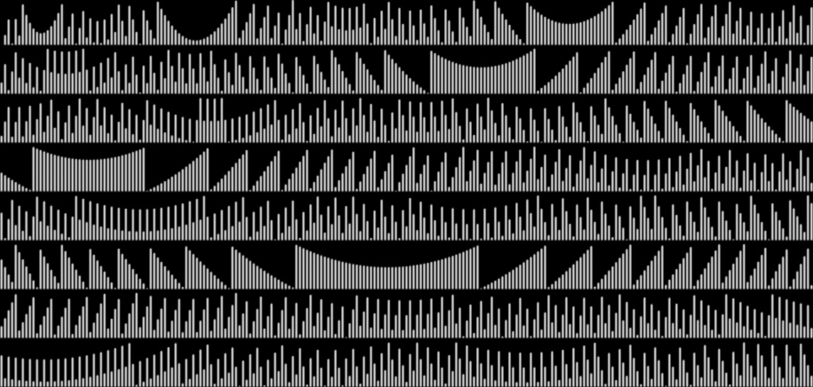
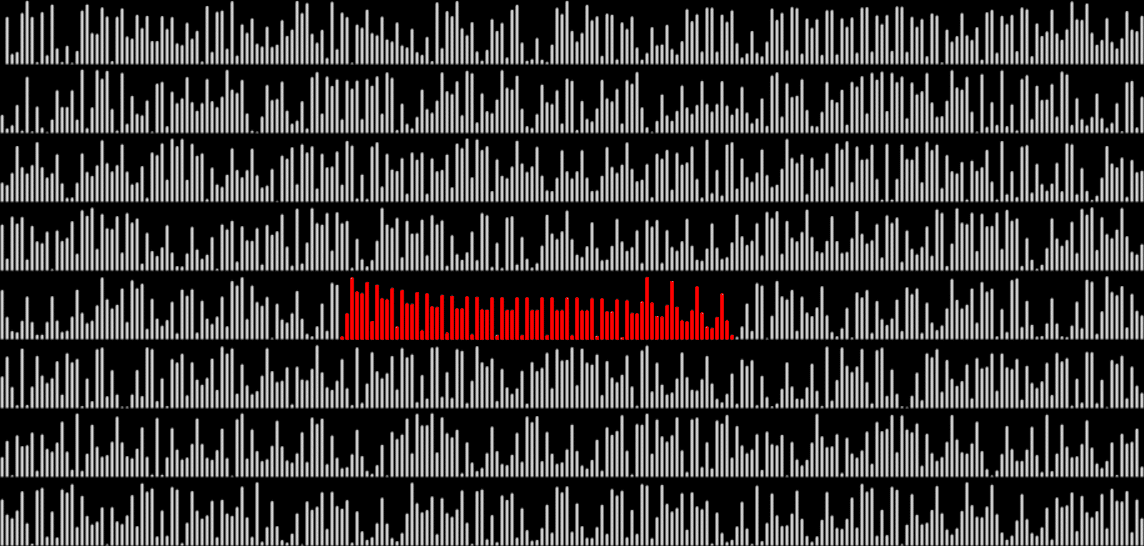
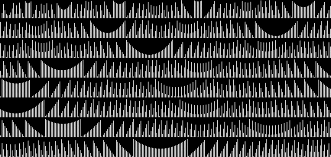
If you want a good example of how, in math, something very simple can quickly get very deep, just look at partitions. Here are the partitions of 1 to 5, that is, the ways 1 to 5 can be expressed as a sum of integers smaller than or equal to themselves:
1 = 1

numbpart(1) = 1


2 = 2
1 + 1 = 2

numbpart(2) = 2


3 = 3
1 + 2 = 3
1 + 1 + 1 = 3

numbpart(3) = 3


4 = 4
1 + 3 = 4
2 + 2 = 4
1 + 1 + 2 = 4
1 + 1 + 1 + 1 = 4

numbpart(4) = 5


5 = 5
1 + 4 = 5
2 + 3 = 5
1 + 1 + 3 = 5
1 + 2 + 2 = 5
1 + 1 + 1 + 2 = 5
1 + 1 + 1 + 1 + 1 = 5

numbpart(5) = 7


It’s very easy to understand the concept of partitions, but very difficult to understand how partitions behave. For example, here is numbpart(n), the count of partitions for 1, 2, 3,…

1, 2, 3, 5, 7, 11, 15, 22, 30, 42, 56, 77, 101, 135, 176, 231, 297, 385, 490, 627, 792, 1002, 1255, 1575, 1958, 2436, 3010, 3718, 4565, 5604, 6842, 8349, 10143, 12310, 14883, 17977, 21637, 26015, 31185, 37338, 44583, 53174, 63261, 75175, 89134, 105558, 124754, 147273, 173525, 204226, … A000041 at the Online Encyclopedia of Integer Sequences, “a(n) is the number of partitions of n (the partition numbers)”

What’s the formula for numbpart(n)? That’s a tricky question. And what’s the formula for the curves produced by counting the various lengths of partitions(n)? That’s another tricky question, but one thing is easy to see. As n gets bigger, the graph of countlen(partitions(n)) acquires a strange, lopsided beauty. Here are the partitions of 8, with the count of how many partitions of a particular length there are:

8 = 8 (1 partition of length 1)
1 + 7 = 8
2 + 6 = 8
3 + 5 = 8
4 + 4 = 8 (4 partitions of length 2)
1 + 1 + 6 = 8
1 + 2 + 5 = 8
1 + 3 + 4 = 8
2 + 2 + 4 = 8
2 + 3 + 3 = 8 (5 of length 3)
1 + 1 + 1 + 5 = 8
1 + 1 + 2 + 4 = 8
1 + 1 + 3 + 3 = 8
1 + 2 + 2 + 3 = 8
2 + 2 + 2 + 2 = 8 (5 of length 4)
1 + 1 + 1 + 1 + 4 = 8
1 + 1 + 1 + 2 + 3 = 8
1 + 1 + 2 + 2 + 2 = 8 (3 of length 5)
1 + 1 + 1 + 1 + 1 + 3 = 8
1 + 1 + 1 + 1 + 2 + 2 = 8 (2 of length 6)
1 + 1 + 1 + 1 + 1 + 1 + 2 = 8 (1 of length 7)
1 + 1 + 1 + 1 + 1 + 1 + 1 + 1 = 8 (1 of length 8)

When counts like that are shown as a graph, the graphs look like this (maximum counts are normalized to the same height):


graph of countlen(partitions(2))


countlen(partitions(3))


countlen(partitions(4))


countlen(partitions(5))


countlen(partitions(6))


countlen(partitions(7))


countlen(partitions(8))


countlen(partitions(9))


countlen(partitions(10))


countlen(partitions(15))


countlen(partitions(20))


countlen(partitions(30))


countlen(partitions(40))


countlen(partitions(50))


countlen(partitions(60))


countlen(partitions(70))


countlen(partitions(80))


countlen(partitions(90))


countlen(partitions(100))


Animated gif of partlen graphs (courtesy EZgif)


The graphs have a long, low right tail because the counts rise to great heights very quick, then fall away again, as you can see with partitions(100):

1 = count(partitions(10),len=1)
50 = count(partitions(10),len=2)
833 = count(partitions(10),len=3)
7153 = count(partitions(10),len=4)
38225 = count(partitions(10),len=5)
143247 = count(partitions(10),len=6)

[…]

10643083 = count(partitions(10),len=16)
11022546 = count(partitions(10),len=17)
11087828 = count(partitions(10),len=18)
10885999 = count(partitions(10),len=19)
10474462 = count(partitions(10),len=20)

[…]

30 = count(partitions(10),len=91)
22 = count(partitions(10),len=92)
15 = count(partitions(10),len=93)
11 = count(partitions(10),len=94)
7 = count(partitions(10),len=95)
5 = count(partitions(10),len=96)
3 = count(partitions(10),len=97)
2 = count(partitions(10),len=98)
1 = count(partitions(10),len=99)
1 = count(partitions(10),len=100)