Deep-Dive Dyadendricity

This simple equation helps you understand a fractal:

1 + 1/2 + 1/4 + 1/8 + 1/16 + 1/32 + … = 2 = Σ(1/2k,k=0..∞)

Now here’s the construction of the H-tree fractal, in which the lines are divided in length by sqrt(2) = 1.41421356237… at each stage. Or multiplied by 0.70710678118… = &sqrt;0.5. This means that, after two divisions, the lines are 1/2 the size. So in the end they create a 1 x &sqrt;2 rectangle:

H-Tree fractal #1


H-Tree fractal #2


H-Tree fractal #3


H-Tree fractal #4


H-Tree fractal #5


H-Tree fractal #6


H-Tree fractal #7


H-Tree fractal #8


H-Tree fractal #9


H-Tree fractal #10


[…]

H-Tree fractal #13


H-Tree fractal #14


H-Tree fractal #15


Here’s an animation:

H-Tree fractal (animated at EZgif)


And here’s the H-tree in black-and-white:

H-Tree fractal #3

H-Tree fractal #6

H-Tree fractal #6

H-Tree fractal #12

H-Tree fractal #15

H-Tree fractal (animated at EZgif)


Because the construction of the H-tree is governed by a string of directions — for example, left-right-right-left-left-left… or 211222… — you can perform tests on that string to create sub-fractals from the super-fractal. Like this:

count(1) = count(2) in string to step 12


count(1) = count(2) in string (omitting lines)


sum(string) = mul(string)


sum(string) > mul(string)


count(1) = 2 or count(2) = 2 after step 2


count(1) < count(2)


count(1) < 3 or count(2) < 3 after step 6


value of string after step 8 > value of string at step 1


value after step 8 > value at step 4


value after step 8 < value step 1


ispalindrome(string) to step 11


ispalindrome(string) to step 18


ispalindrome(string) to step 20


alternating 121… or 212… in string after step 9


ispolygonal(sum(string[i]-1),pol=10)


isprime(sum(string))


sum(string[i]-1) mod 13 = 0


sum(string[i]-1) mod 13 = 1


sum(string[i]-1) mod 16 = 0


sum(string[i]-1) mod 18 = 0


Mathematicoynte

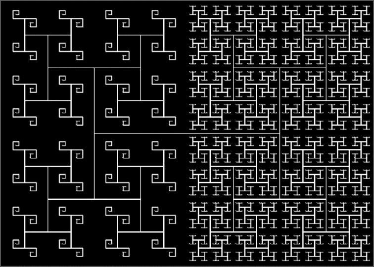
Pre-previously, I looked at a fractal phallus. Now I want to look at a fractal fanny (in the older British sense). In fact, it’s a fractional fractal fanny. Take a look at these fractions:


1/10, 1/9, 1/8, 1/7, 1/6, 1/5, 2/10, 2/9, 1/4, 2/8, 2/7, 3/10, 1/3, 2/6, 3/9, 3/8, 2/5, 4/10, 3/7, 4/9, 1/2, 2/4, 3/6, 4/8, 5/10, 5/9, 4/7, 3/5, 6/10, 5/8, 2/3, 4/6, 6/9, 7/10, 5/7, 3/4, 6/8, 7/9, 4/5, 8/10, 5/6, 6/7, 7/8, 8/9, 9/10

They’re all the fractions for 1/2..(n-1)/n, n = 10, sorted by increasing size. But obviously some of them are the same: 1/2 = 2/4 = 3/6 = 5/10, 1/3 = 2/6 = 3/9, 1/4 = 2/8, and so on. If you remove the duplicates, you get this set of reduced fractions:


1/10, 1/9, 1/8, 1/7, 1/6, 1/5, 2/9, 1/4, 2/7, 3/10, 1/3, 3/8, 2/5, 3/7, 4/9, 1/2, 5/9, 4/7, 3/5, 5/8, 2/3, 7/10, 5/7, 3/4, 7/9, 4/5, 5/6, 6/7, 7/8, 8/9, 9/10

Now here are the reduced fractions for 1/2..(n-1)/n, n = 30:


1/30, 1/29, 1/28, 1/27, 1/26, 1/25, 1/24, 1/23, 1/22, 1/21, 1/20, 1/19, 1/18, 1/17, 1/16, 1/15, 2/29, 1/14, 2/27, 1/13, 2/25, 1/12, 2/23, 1/11, 2/21, 1/10, 3/29, 2/19, 3/28, 1/9, 3/26, 2/17, 3/25, 1/8, 3/23, 2/15, 3/22, 4/29, 1/7, 4/27, 3/20, 2/13, 3/19, 4/25, 1/6, 5/29, 4/23, 3/17, 5/28, 2/11, 5/27, 3/16, 4/21, 5/26, 1/5, 6/29, 5/24, 4/19, 3/14, 5/23, 2/9, 5/22, 3/13, 7/30, 4/17, 5/21, 6/25, 7/29, 1/4, 7/27, 6/23, 5/19, 4/15, 7/26, 3/11, 8/29, 5/18, 7/25, 2/7, 7/24, 5/17, 8/27, 3/10, 7/23, 4/13, 9/29, 5/16, 6/19, 7/22, 8/25, 9/28, 1/3, 10/29, 9/26, 8/23, 7/20, 6/17, 5/14, 9/25, 4/11, 11/30, 7/19, 10/27, 3/8, 11/29, 8/21, 5/13, 7/18, 9/23, 11/28, 2/5, 11/27, 9/22, 7/17, 12/29, 5/12, 8/19, 11/26, 3/7, 13/30, 10/23, 7/16, 11/25, 4/9, 13/29, 9/20, 5/11, 11/24, 6/13, 13/28, 7/15, 8/17, 9/19, 10/21, 11/23, 12/25, 13/27, 14/29, 1/2, 15/29, 14/27, 13/25, 12/23, 11/21, 10/19, 9/17, 8/15, 15/28, 7/13, 13/24, 6/11, 11/20, 16/29, 5/9, 14/25, 9/16, 13/23, 17/30, 4/7, 15/26, 11/19, 7/12, 17/29, 10/17, 13/22, 16/27, 3/5, 17/28, 14/23, 11/18, 8/13, 13/21, 18/29, 5/8, 17/27, 12/19, 19/30, 7/11, 16/25, 9/14, 11/17, 13/20, 15/23, 17/26, 19/29, 2/3, 19/28, 17/25, 15/22, 13/19, 11/16, 20/29, 9/13, 16/23, 7/10, 19/27, 12/17, 17/24, 5/7, 18/25, 13/18, 21/29, 8/11, 19/26, 11/15, 14/19, 17/23, 20/27, 3/4, 22/29, 19/25, 16/21, 13/17, 23/30, 10/13, 17/22, 7/9, 18/23, 11/14, 15/19, 19/24, 23/29, 4/5, 21/26, 17/21, 13/16, 22/27, 9/11, 23/28, 14/17, 19/23, 24/29, 5/6, 21/25, 16/19, 11/13, 17/20, 23/27, 6/7, 25/29, 19/22, 13/15, 20/23, 7/8, 22/25, 15/17, 23/26, 8/9, 25/28, 17/19, 26/29, 9/10, 19/21, 10/11, 21/23, 11/12, 23/25, 12/13, 25/27, 13/14, 27/29, 14/15, 15/16, 16/17, 17/18, 18/19, 19/20, 20/21, 21/22, 22/23, 23/24, 24/25, 25/26, 26/27, 27/28, 28/29, 29/30

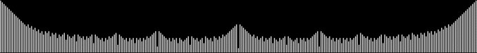
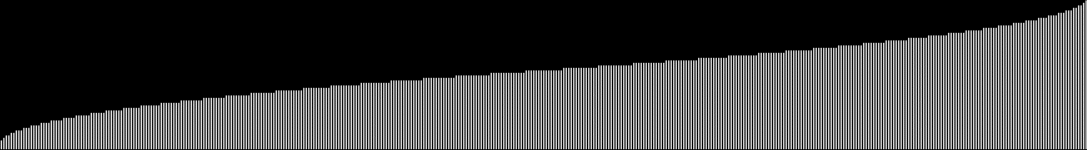
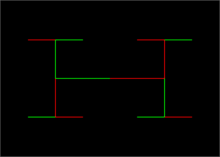
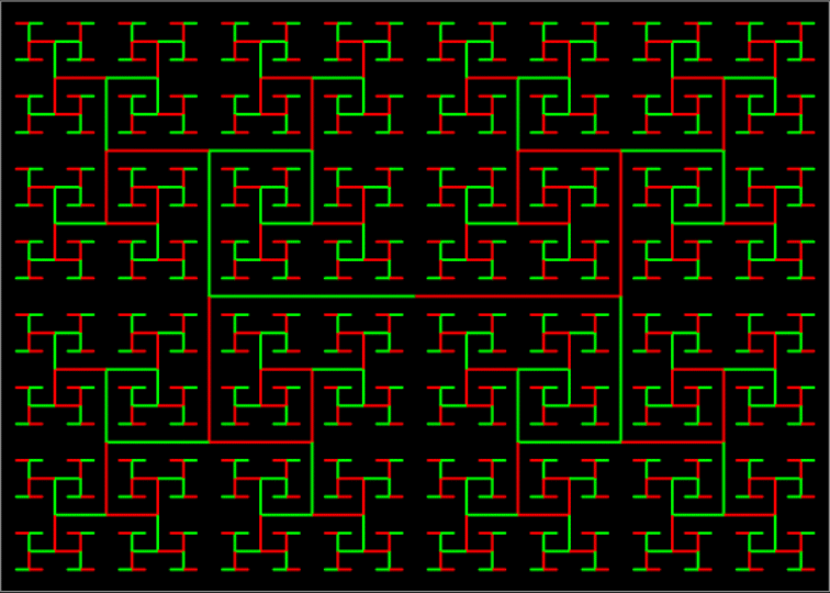
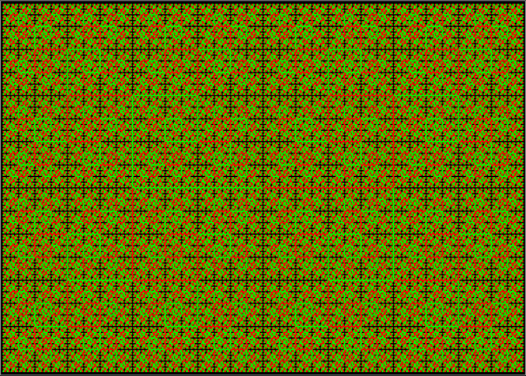
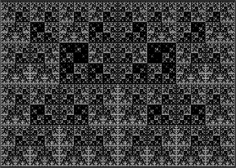
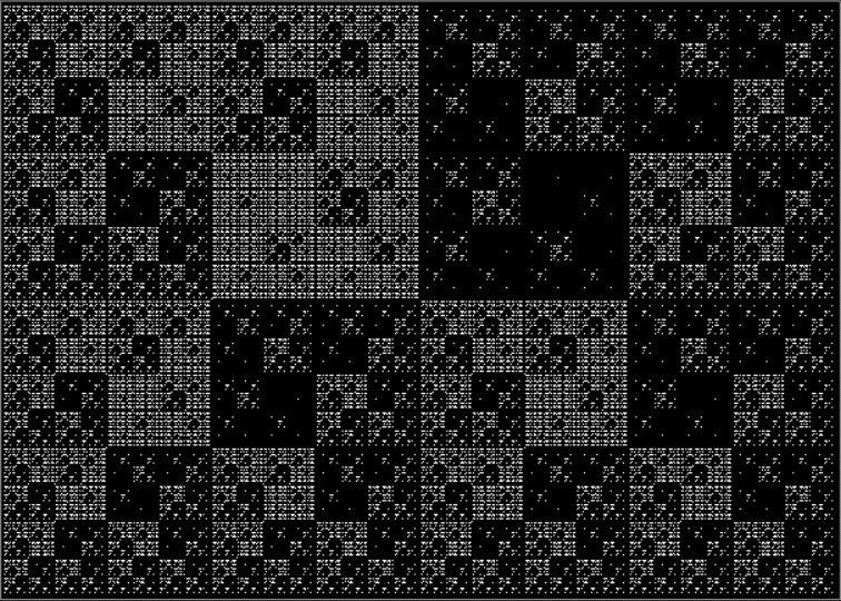
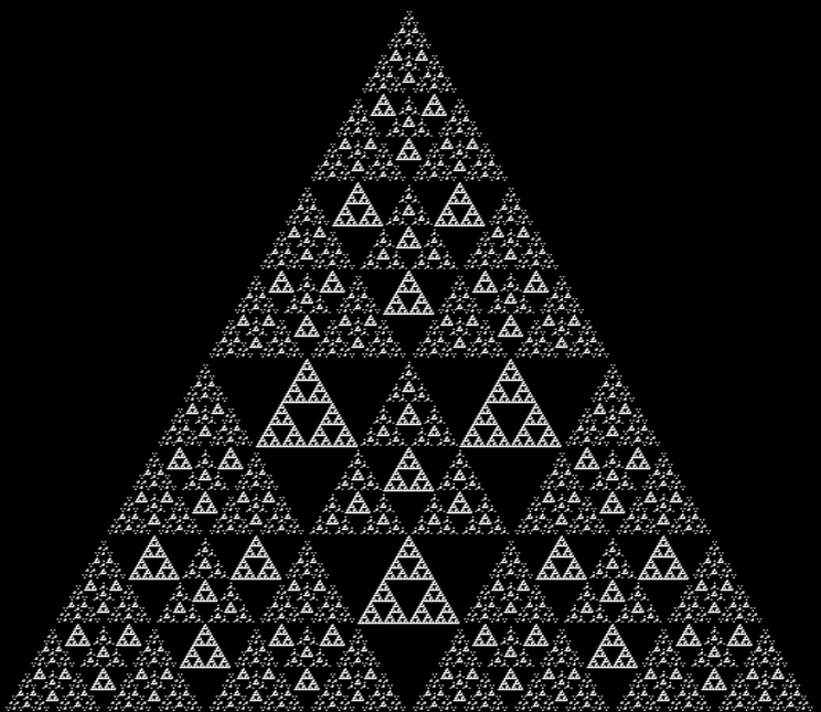
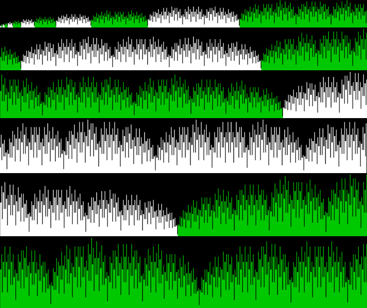
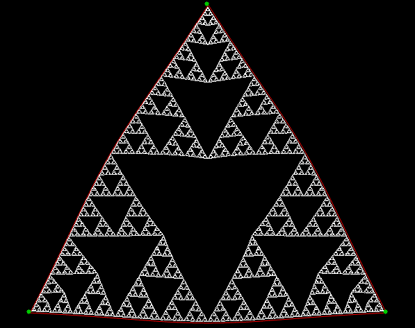
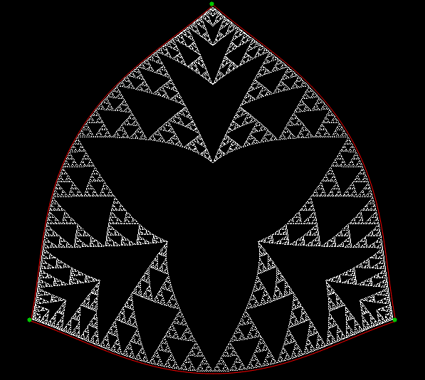
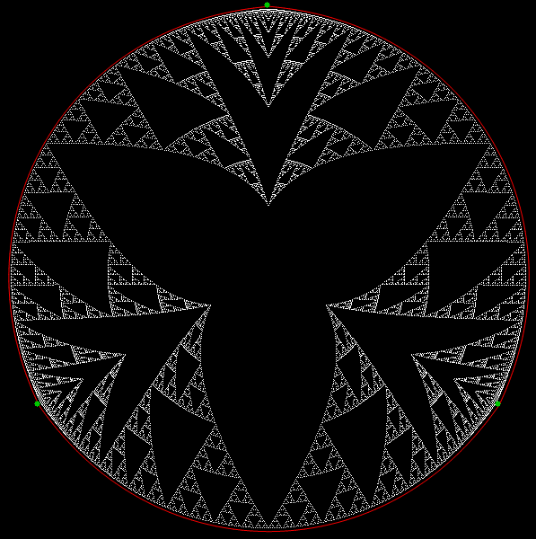
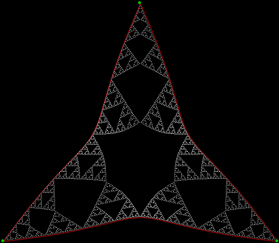
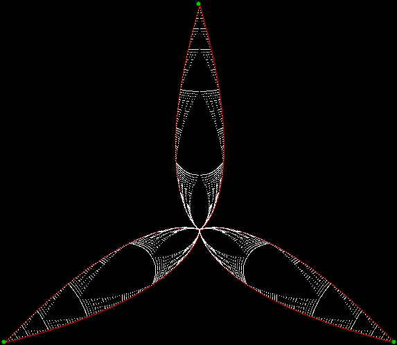
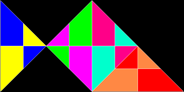
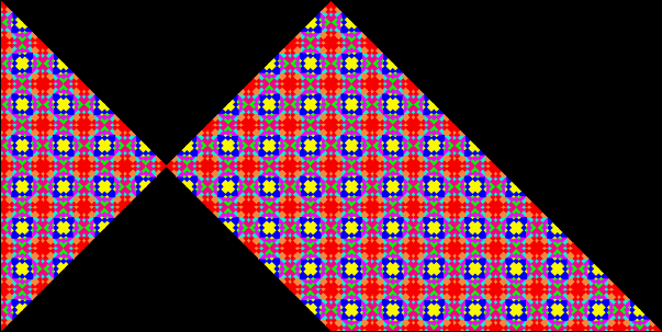
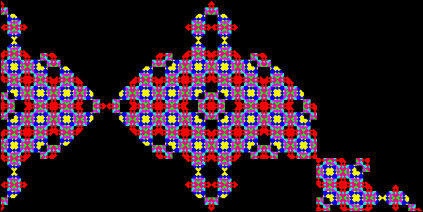
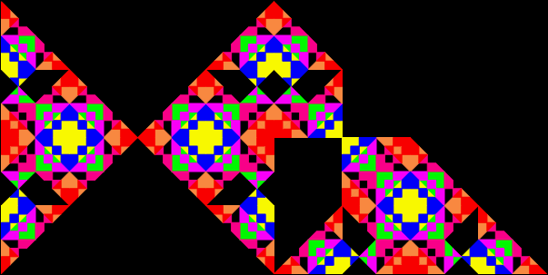
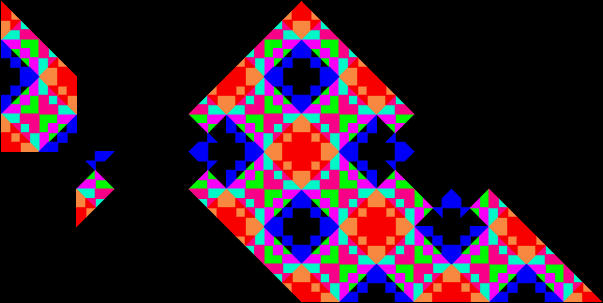
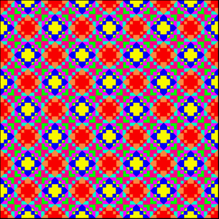
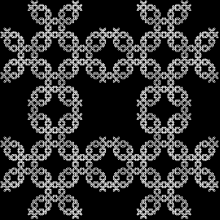
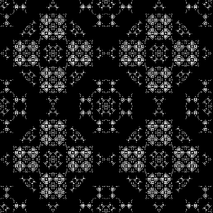
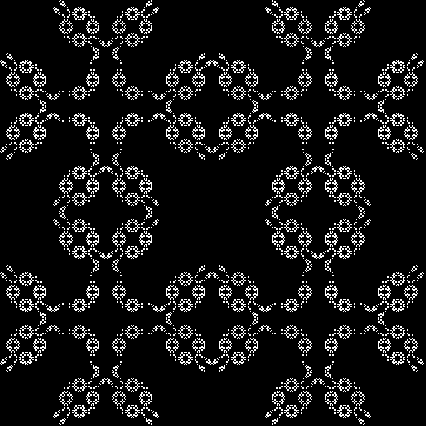
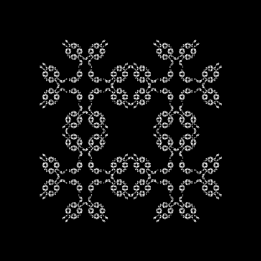
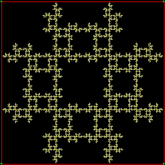
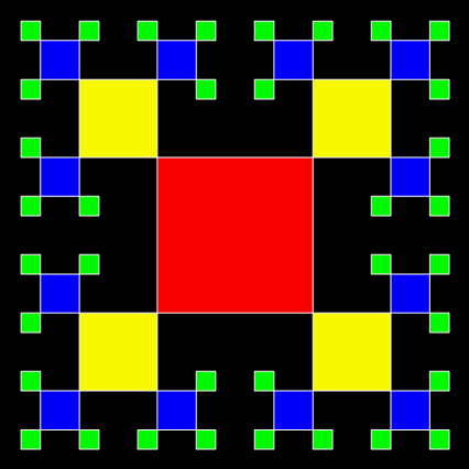
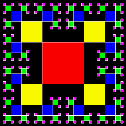
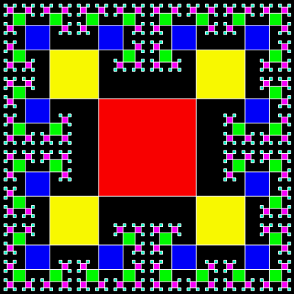
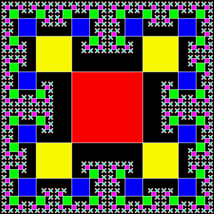
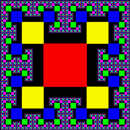
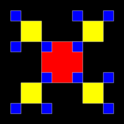
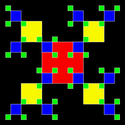
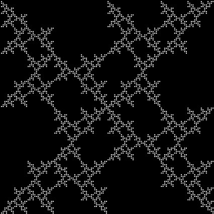
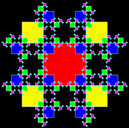
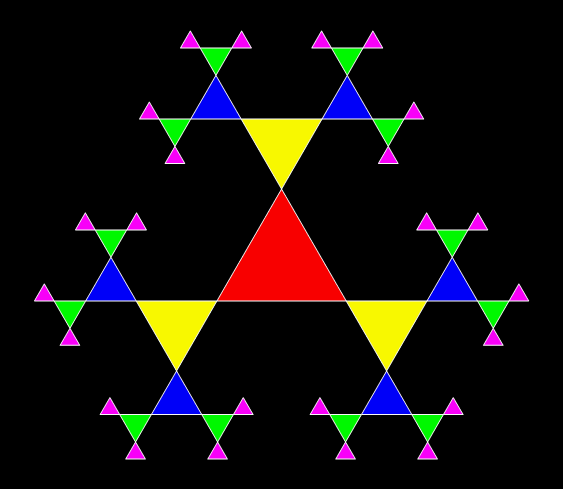
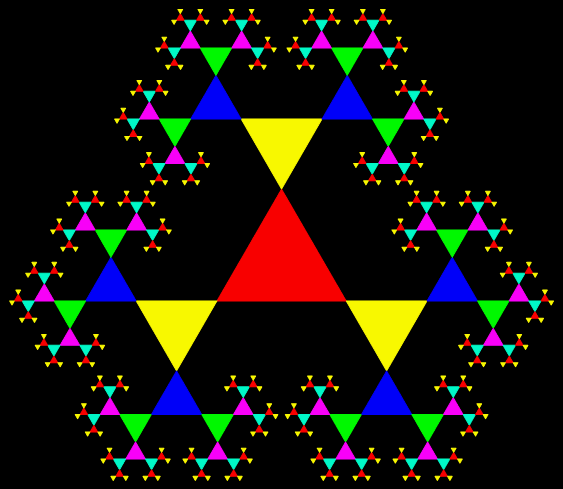
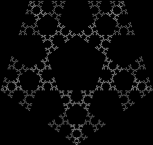
Can you see the fractal fanny? Not unless you’re superhuman. But any normal human can see the fractal fanny when you turn those reduced and sorted fractions, a/b, into a graph, where y = b and x = n for a/bn:

graph for b of reduced a/b = 1/2..29/30, sorted by size of a/b

(click for larger)


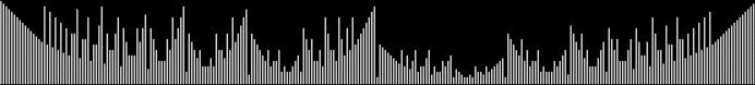
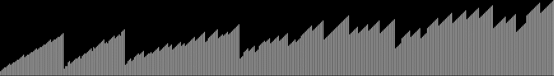
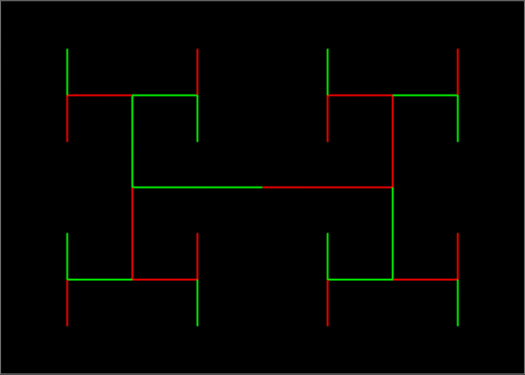
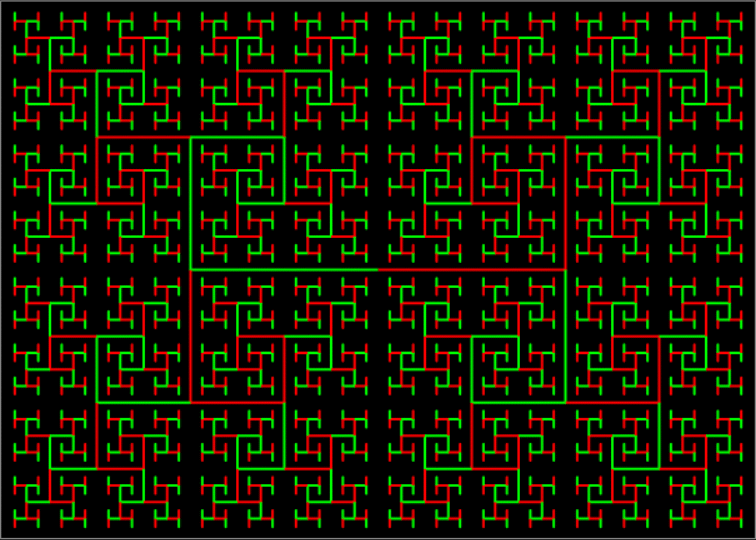
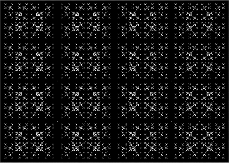
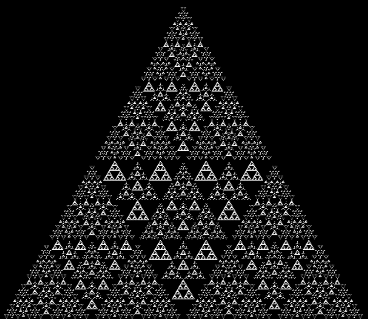
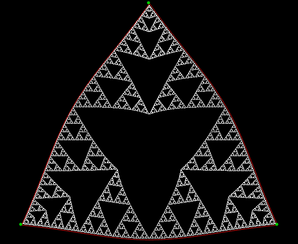
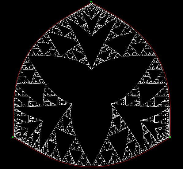
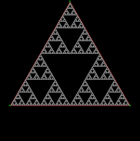
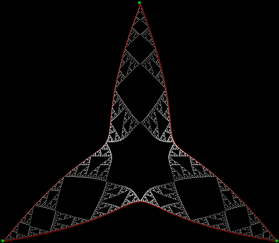
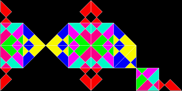
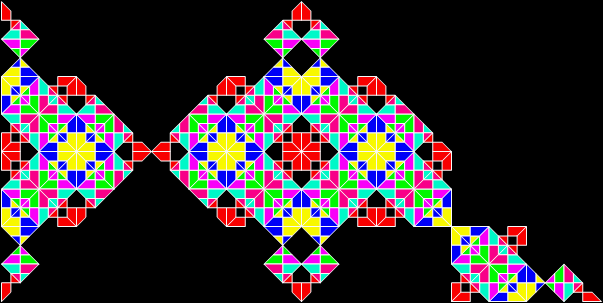
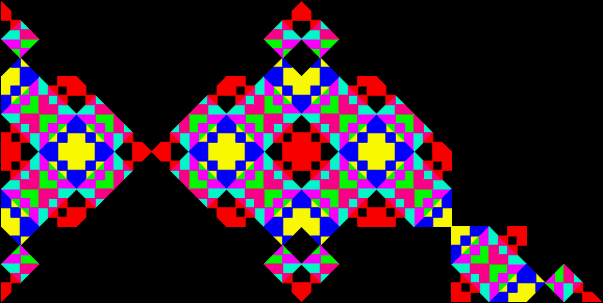
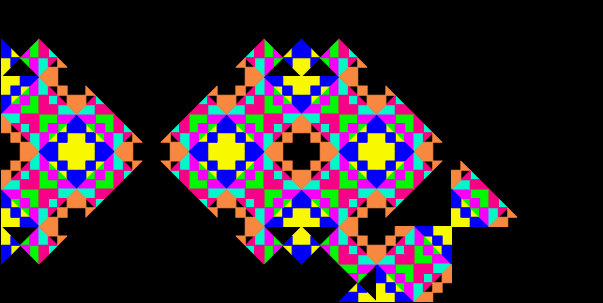
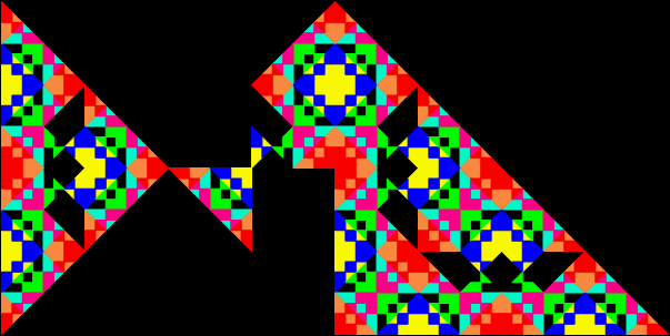
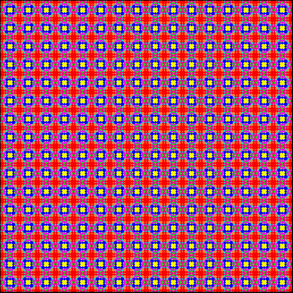
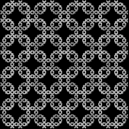
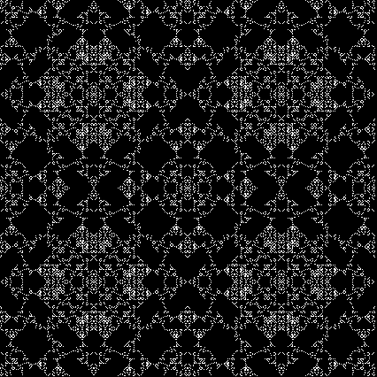
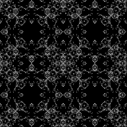
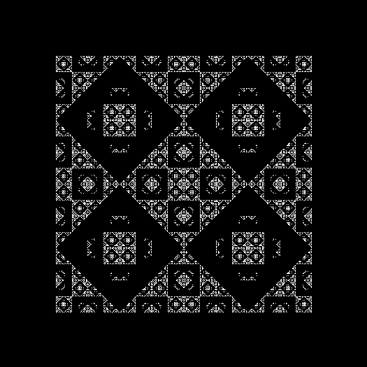
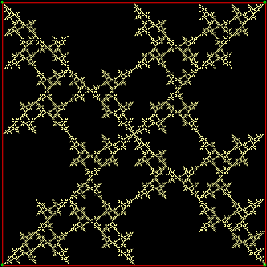
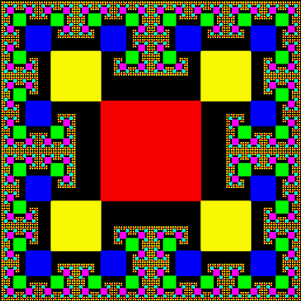
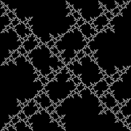
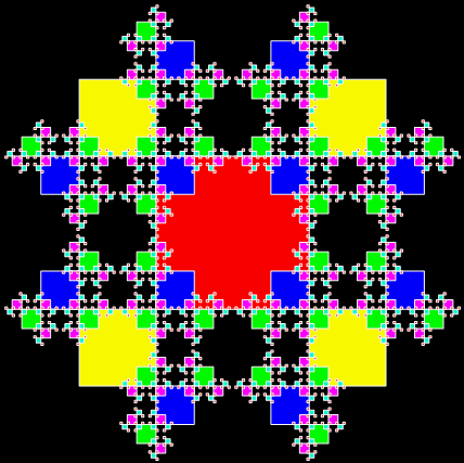
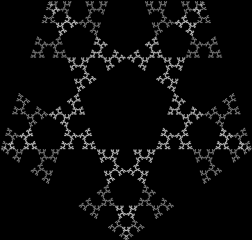
If you don’t reduce the fractions, you get this distorted coynte:

graph for b of all fractions 1/2..29/30, sorted by a/b


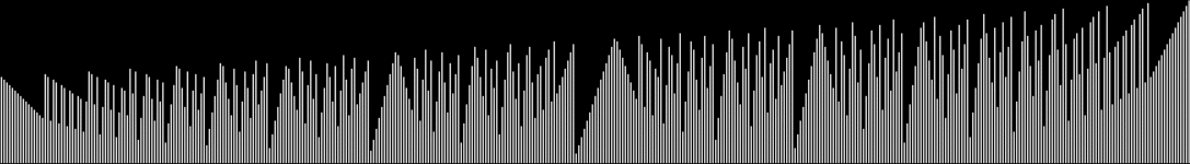
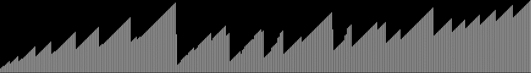
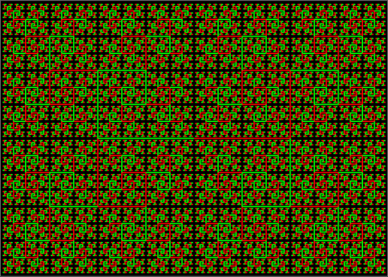
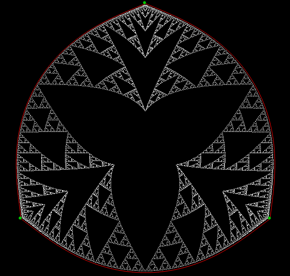
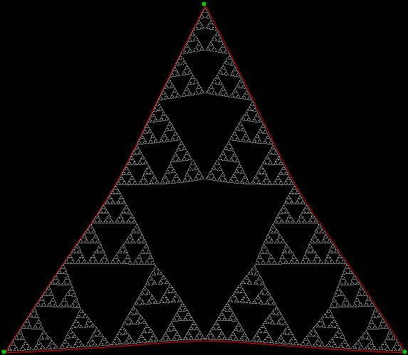
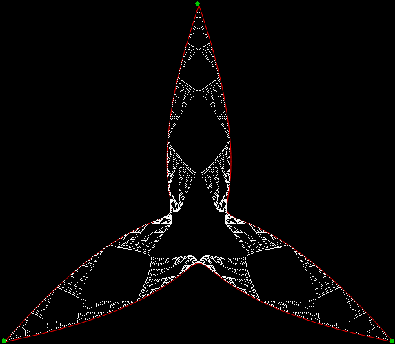
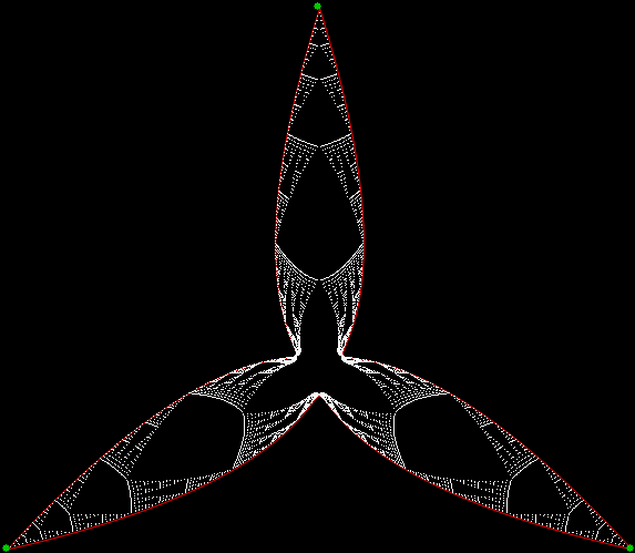
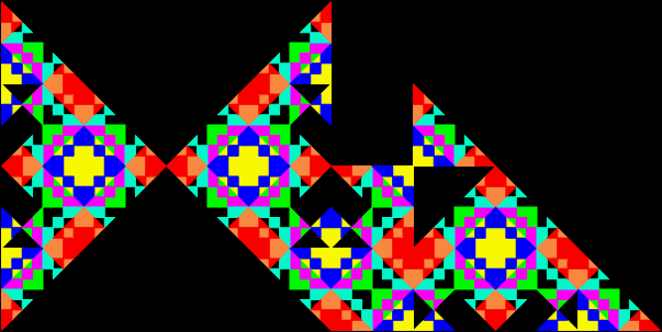
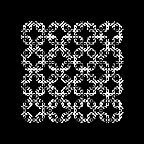
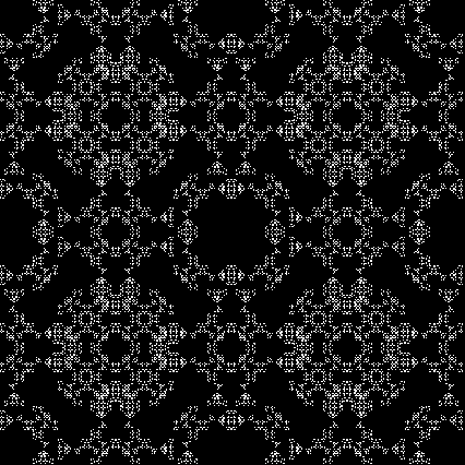
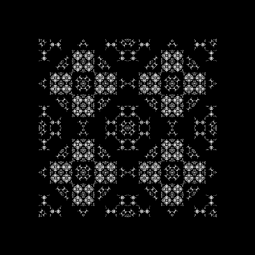
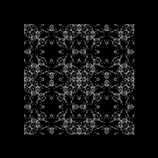
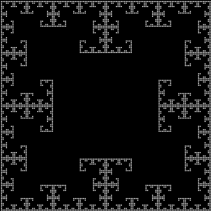
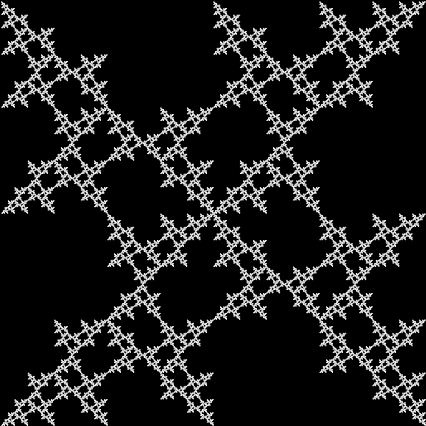
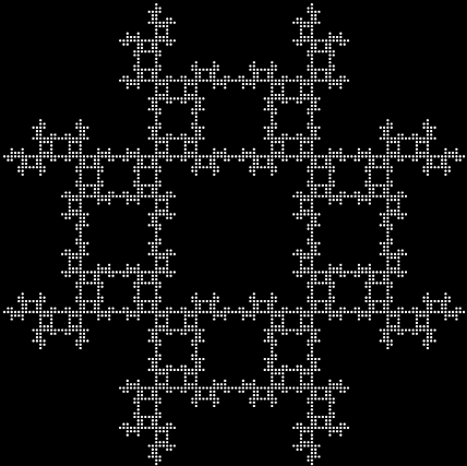
And you can use other variables for y, like the sum of the continued fraction of a/b:

graph for sum(contfrac(a/b)) of reduced fractions 1/2..29/30, sorted by a/b


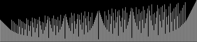
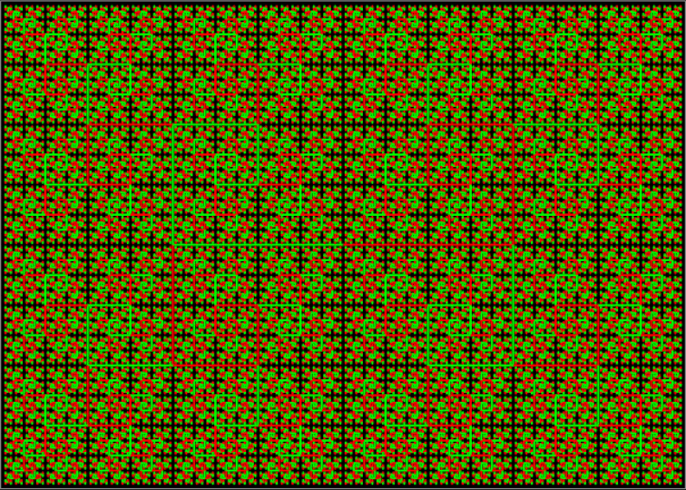
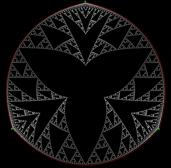
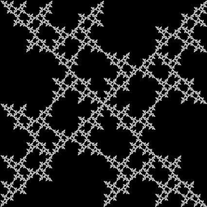
graph for cfsum of all fractions 1/2..29/30, sorted by a/b


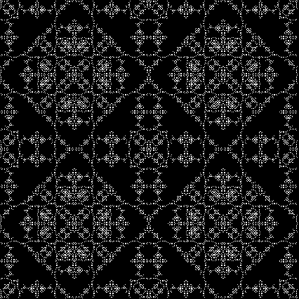
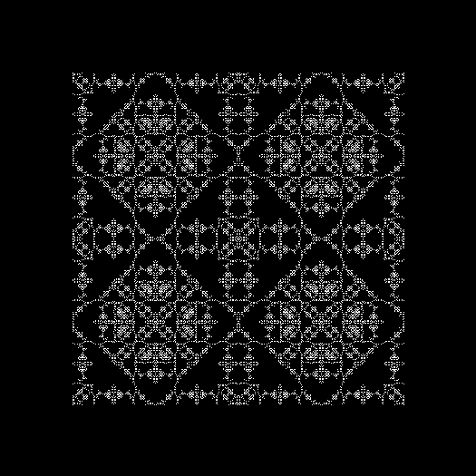
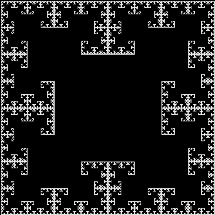
And the product of the continued fraction of a/b:

graph for prod(contfrac(a/b)) of reduced fractions 1/2..29/30, sorted by a/b


graph for cfmul of all fractions 1/2..29/30, sorted by a/b


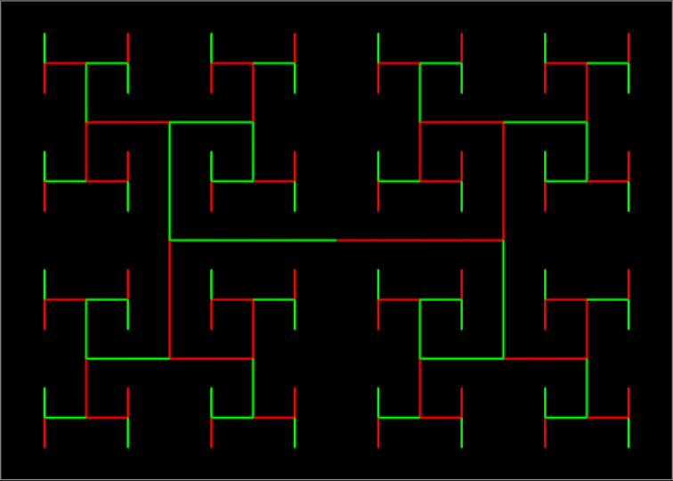
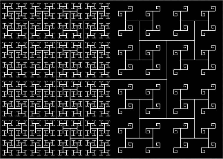
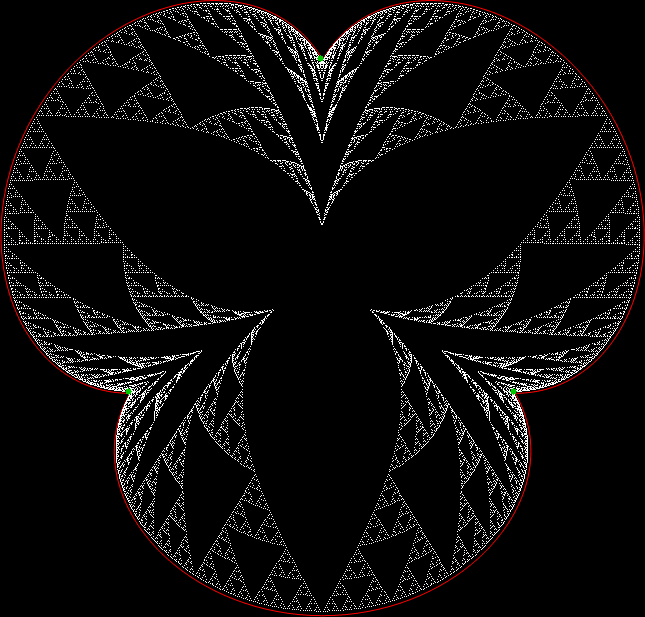
And you can sort by the size of other variables, like the number of factors of b:

graph for a+b of all fractions 1/2..29/30, sorted by factornum(b)
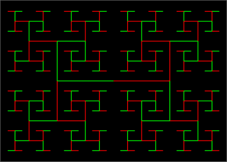
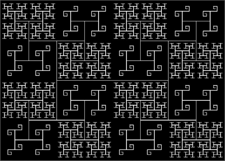

And so on:

graph for a of reduced fractions 1/2..29/30, sorted by a/b


graph for a of reduced fractions 1/2..29/30, sorted by a/b


graph for a of all fractions 1/2..29/30, sorted by a/b


graph for a of all fractions 1/2..29/30, sorted by length(contfrac(a/b))


graph for a of all fractions 1/2..29/30, sorted by factornum(b)


graph for a of all fractions 1/2..29/30, sorted by gcd(a/b)


graph for a+b of all fractions 1/2..29/30, sorted by a/b


graph for a+b of reduced fractions 1/2..29/30, sorted by a/b


graph for a+b of all fractions 1/2..29/30, sorted by a+b


graph for a+b of all fractions 1/2..29/30, sorted by cflen(a/b)


graph for a+b of all fractions 1/2..29/30, sorted by gbd(a,b)


graph for b of all fractions 1/2..29/30, sorted by a+b


graph for b of all fractions 1/2..29/30, sorted by cflen(a/b)


graph for b of all fractions 1/2..29/30, sorted by factnum(b)


graph for b of all fractions 1/2..29/30, sorted by gcd(a,b)


graph for b-a of all fractions 1/2..29/30, sorted by a/b


graph for b-a of reduced fractions 1/2..29/30, sorted by a/b


graph for b-a of all fractions 1/2..29/30, sorted by a+b


graph for b-a of all fractions 1/2..29/30, sorted by factnum(b)


graph for cfmul of all fractions 1/2..29/30, sorted by a


graph for cfsum of all fractions 1/2..29/30, sorted by a


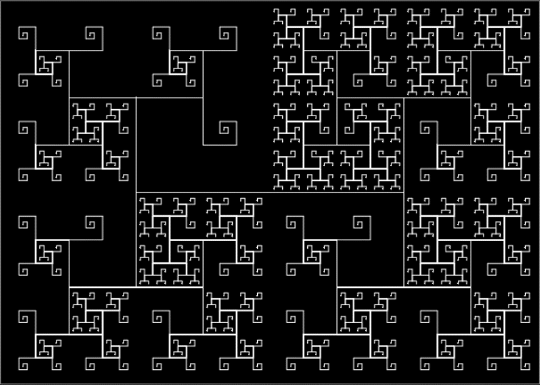
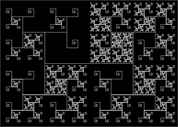
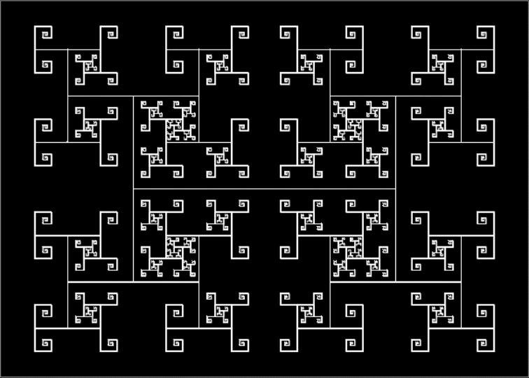
Previously Pre-Posted (Please Peruse)

Phrallic Frolics — a look at fractal phalluses, a.k.a. phralluses

Mods and Clockers

To understand clock-arithmetic, simply picture a clock-face with one hand and a big fat 0 in place of the 12. Now you can do some clock-arithmetic. For example, set the hour-hand to 5, then move on 4 hours. You’ve done this sum:

5 + 4 → 9

Now try 9 + 7. The hour-hand is already on 9, so move forward 7 hours:

9 + 7 → 4

Now try 3 + 8 + 1:

3 + 8 + 1 → 0

And 3 * 4:

4 * 3 = 4 + 4 + 4 → 0

That’s clock-arithmetic. But you’re not confined to 12-hour clocks. Here’s a 7-hour clock, where the 7 is replaced with a 0:

3 + 1 → 4
4 + 5 → 2
2 + 4 + 1 → 0
3 * 3 = 3 + 3 + 3 → 2

Another name for clock-arithmetic is modular arithmetic, because the clocks model the process of dividing a number by 12 or 7 and finding the remainder or residue — 12 or 7 is known as the modulus (and modulo is Latin for “by the modulus”).

5 + 4 = 9 → 9 / 12 = 0*12 + 9

(5 + 4) modulo 12 = 9


3 + 8 + 1 = 12 → 12 / 12 = 1*12 + 0

(3 + 8 + 1) modulo 12 = 0


19 / 12 = 1*12 + 7

19 mod 12 = 7


3 + 1 = 4 → 4 / 7 = 0*7 + 4

(3 + 1) mod 7 = 4


2 + 4 + 1 = 7 → 7 / 7 = 1*7 + 0

(2 + 4 + 1) mod 7 = 0


19 / 7 = 2*7 + 5

19 mod 7 = 5


Modular arithmetic can do wonderful things. One small but beautiful example is the way it can uncover hidden fractals in Pascal’s triangle:

Pascal’s Triangle (via Desmos)


How to create Pascal’s triangle (via Wikipedia)


If you color all numbers n mod 2 = 1 (i.e., odd numbers) in the triangle, they create the famous Sierpiński triangle:

The Sierpiński triangle in Pascal’s triangle (via Fractal Foundation)

Pascal’s triangle, n mod 2 = 1 (click for larger)


The Sierpiński triangle appears like this for all n mod 4 = 2 in Pascal’s triangle:

Pascal’s triangle, n mod 4 = 2 (click for larger)


And so on:

Pascal’s triangle, n mod 8 = 4


Pascal’s triangle, n mod 16 = 8


Pascal’s triangle, n mod 32 = 16


Pascal’s triangle, n mod 64 = 32


Pascal’s triangle, n mod 128 = 64


Pascal’s triangle, n mod 256 = 128


Pascal’s triangle, n mod 2,4,8… = 1,2,4… (animated via EzGif)


Post-Performative Post-Scriptum

There’s no need to calculate Pascal’s triangle in full to find the fractals above. The 10th row of Pascal’s triangle is this:

1, 10, 45, 120, 210, 252, 210, 120, 45, 10, 1

The 20th row is this:

1, 20, 190, 1140, 4845, 15504, 38760, 77520, 125970, 167960, 184756, 167960, 125970, 77520, 38760, 15504, 4845, 1140, 190, 20, 1

And the 29th is this:

1, 29, 406, 3654, 23751, 118755, 475020, 1560780, 4292145, 10015005, 20030010, 34597290, 51895935, 67863915, 77558760, 77558760, 67863915, 51895935, 34597290, 20030010, 10015005, 4292145, 1560780, 475020, 118755, 23751, 3654, 406, 29, 1

But you don’t need to consider those ever-growing numbers in the triangle when you’re finding fractals with modular arithmetic. When the modulus is 2, you just work with 0 and 1, that is, you add the previous numbers in the triangle and find the sum modulo 2. When the modulus is 4, you just work with 0, 1, 2 and 3, adding the numbers and finding the sum modulo 4. When it’s 8, you just work with 0, 1, 2, 3, 4, 5, 6 and 7, finding the sum modulo 8. And so on.

Fabulous Furry Fibonacci Fractal

At least, I think it’s a fractal. I came across it when I was counting the ways in which the integers can be the sum of distinct Fibonacci numbers. Here for reference is the Fibonacci sequence, the beautiful and endlessly fertile sequence that’s seeded with “1, 1” and continued by summing the two previous numbers:

1, 1, 2, 3, 5, 8, 13, 21, 34, 55, 89, 144, 233, 377, 610, 987, 1597, 2584, 4181, 6765, 10946, 17711, 28657, 46368, 75025, 121393, 196418, 317811, 514229, 832040…

I noticed some interesting patterns in the distinct-fib-num-sum count for the integers:

1 = 1 (count=1)
2 = 2 (count=1)
3 = 1+2 = 3 (count=2)
4 = 1+3 (c=1)
5 = 2+3 = 5 (c=2)
6 = 1+2+3 = 1+5 (c=2)
7 = 2+5 (c=1)
8 = 1+2+5 = 3+5 = 8 (c=3)
9 = 1+3+5 = 1+8 (c=2)
10 = 2+3+5 = 2+8 (c=2)
11 = 1+2+3+5 = 1+2+8 = 3+8 (c=3)
12 = 1+3+8 (c=1)
13 = 2+3+8 = 5+8 = 13 (c=3)
14 = 1+2+3+8 = 1+5+8 = 1+13 (c=3)
15 = 2+5+8 = 2+13 (c=2)
16 = 1+2+5+8 = 3+5+8 = 1+2+13 = 3+13 (c=4)
17 = 1+3+5+8 = 1+3+13 (c=2)
18 = 2+3+5+8 = 2+3+13 = 5+13 (c=3)
19 = 1+2+3+5+8 = 1+2+3+13 = 1+5+13 (c=3)
20 = 2+5+13 (c=1)
21 = 1+2+5+13 = 3+5+13 = 8+13 = 21 (c=4)
22 = 1+3+5+13 = 1+8+13 = 1+21 (c=3)
23 = 2+3+5+13 = 2+8+13 = 2+21 (c=3)
24 = 1+2+3+5+13 = 1+2+8+13 = 3+8+13 = 1+2+21 = 3+21 (c=5)
25 = 1+3+8+13 = 1+3+21 (c=2)
26 = 2+3+8+13 = 5+8+13 = 2+3+21 = 5+21 (c=4)
27 = 1+2+3+8+13 = 1+5+8+13 = 1+2+3+21 = 1+5+21 (c=4)
28 = 2+5+8+13 = 2+5+21 (c=2)
29 = 1+2+5+8+13 = 3+5+8+13 = 1+2+5+21 = 3+5+21 = 8+21 (c=5)
30 = 1+3+5+8+13 = 1+3+5+21 = 1+8+21 (c=3)
31 = 2+3+5+8+13 = 2+3+5+21 = 2+8+21 (c=3)
32 = 1+2+3+5+8+13 = 1+2+3+5+21 = 1+2+8+21 = 3+8+21 (c=4)
33 = 1+3+8+21 (c=1)
34 = 2+3+8+21 = 5+8+21 = 13+21 = 34 (c=4)
35 = 1+2+3+8+21 = 1+5+8+21 = 1+13+21 = 1+34 (c=4)
36 = 2+5+8+21 = 2+13+21 = 2+34 (c=3)
37 = 1+2+5+8+21 = 3+5+8+21 = 1+2+13+21 = 3+13+21 = 1+2+34 = 3+34
(c=6)
38 = 1+3+5+8+21 = 1+3+13+21 = 1+3+34 (c=3)
39 = 2+3+5+8+21 = 2+3+13+21 = 5+13+21 = 2+3+34 = 5+34 (c=5)
40 = 1+2+3+5+8+21 = 1+2+3+13+21 = 1+5+13+21 = 1+2+3+34 = 1+5+34
(c=5)
41 = 2+5+13+21 = 2+5+34 (c=2)
42 = 1+2+5+13+21 = 3+5+13+21 = 8+13+21 = 1+2+5+34 = 3+5+34 = 8+3
4 (c=6)
43 = 1+3+5+13+21 = 1+8+13+21 = 1+3+5+34 = 1+8+34 (c=4)
44 = 2+3+5+13+21 = 2+8+13+21 = 2+3+5+34 = 2+8+34 (c=4)
45 = 1+2+3+5+13+21 = 1+2+8+13+21 = 3+8+13+21 = 1+2+3+5+34 = 1+2+
8+34 = 3+8+34 (c=6)
46 = 1+3+8+13+21 = 1+3+8+34 (c=2)
47 = 2+3+8+13+21 = 5+8+13+21 = 2+3+8+34 = 5+8+34 = 13+34 (c=5)
48 = 1+2+3+8+13+21 = 1+5+8+13+21 = 1+2+3+8+34 = 1+5+8+34 = 1+13+
34 (c=5)
49 = 2+5+8+13+21 = 2+5+8+34 = 2+13+34 (c=3)
50 = 1+2+5+8+13+21 = 3+5+8+13+21 = 1+2+5+8+34 = 3+5+8+34 = 1+2+1
3+34 = 3+13+34 (c=6)
51 = 1+3+5+8+13+21 = 1+3+5+8+34 = 1+3+13+34 (c=3)
52 = 2+3+5+8+13+21 = 2+3+5+8+34 = 2+3+13+34 = 5+13+34 (c=4)
53 = 1+2+3+5+8+13+21 = 1+2+3+5+8+34 = 1+2+3+13+34 = 1+5+13+34 (c=4)
54 = 2+5+13+34 (c=1)
55 = 1+2+5+13+34 = 3+5+13+34 = 8+13+34 = 21+34 = 55 (c=5)
56 = 1+3+5+13+34 = 1+8+13+34 = 1+21+34 = 1+55 (c=4)

The patterns are easier to see when the counts are set out like this:

1, 1, 2, 1, 2, 2, 1, 3, 2, 2, 3, 1, 3, 3, 2, 4, 2, 3, 3, 1, 4, 3, 3, 5, 2, 4, 4, 2, 5, 3, 3, 4, 1, 4, 4, 3, 6, 3, 5, 5, 2, 6, 4, 4, 6, 2, 5, 5, 3, 6, 3, 4, 4, 1, 5, 4, 4, 7, 3, 6, 6, 3, 8, 5, 5, 7, 2, 6, 6, 4, 8, 4, 6, 6, 2, 7, 5, 5, 8, 3, 6, 6, 3, 7, 4, 4, 5, 1, 5, 5, 4, 8, 4, 7, 7, 3, 9, 6, 6, 9, 3, 8, 8, 5, 10, 5, 7, 7, 2, 8, 6, 6, 10, 4, 8, 8, 4, 10, 6, 6, 8, 2, 7, 7, 5, 10, 5, 8, 8, 3, 9, 6, 6, 9, 3, 7, 7, 4, 8, 4, 5, 5, 1, 6, 5, 5, 9, 4, 8, 8… 1… — See A000119, Number of representations of n as a sum of distinct Fibonacci numbers, at the Online Encyclopedia of Integer Sequences (OEIS)

The numbers between each pair of 1s are symmetrical:

1, 2, 1,
1, 2, 2, 1,
1, 3, 2, 2, 3, 1,
1, 3, 3, 2, 4, 2, 3, 3, 1
1, 4, 3, 3, 5, 2, 4, 4, 2, 5, 3, 3, 4, 1

And when fibsumcount(n) = 1, then n = fib(i)-1, i.e. n is one less than a Fibonacci number:

1 = 1 (c=1)
2 = 2 (c=1)
4 = 1+3 (c=1)
7 = 2+5 (c=1)
12 = 1+3+8 (c=1)
20 = 2+5+13 (c=1)
33 = 1+3+8+21 (c=1)
54 = 2+5+13+34 (c=1)
88 = 1+3+8+21+55 (c=1)
143 = 2+5+13+34+89 (c=1)
232 = 1+3+8+21+55+144 (c=1)
376 = 2+5+13+34+89+233 (c=1)
609 = 1+3+8+21+55+144+377 (c=1)
986 = 2+5+13+34+89+233+610 (c=1)
1596 = 1+3+8+21+55+144+377+987 (c=1)
2583 = 2+5+13+34+89+233+610+1597 (c=1)
4180 = 1+3+8+21+55+144+377+987+2584 (c=1)
6764 = 2+5+13+34+89+233+610+1597+4181 (c=1)
10945 = 1+3+8+21+55+144+377+987+2584+6765 (c=1)
17710 = 2+5+13+34+89+233+610+1597+4181+10946 (c=1)
[…]

I also noticed a pattern relating to the maximum count reached in the numbers between the 1s. Suppose the function max(fib(i)-1..fib(i+1)-1) returns the highest count of ways to represent the numbers from fib(i)-1 to fib(i+1)-1. Notice how max() increases:

max(2..4) = 2
max(4..7) = 2
max(7..12) = 3
max(12..20) = 4
max(20..33) = 5
max(33..54) = 6
max(54..88) = 8
max(88..143) = 10
max(143..232) = 13
max(232..376) = 16
max(376..609) = 21
max(609..986) = 26
max(986..1596) = 34
max(1596..2583) = 42
max(2583..4180) = 55
max(4180..6764) = 68
[…]

The pattern is described like this at the Online Encyclopedia of Integer Sequences:

a(n) = 1 if and only if n+1 is a Fibonacci number. The length of such a quasi-period (from Fib(i)-1 to Fib(i+1)-1, inclusive) is a Fibonacci number + 1. The maximum value of a(n) within each subsequent quasi-period increases by a Fibonacci number. For example, from n = 143 to n = 232, the maximum is 13. From 232 to 376, the maximum is 16, an increase of 3. From 376 to 609, 21, an increase of 5. From 609 to 986, 26, increasing by 5 again. Each two subsequent maxima seem to increase by the same increment, the next Fibonacci number. – Kerry Mitchell, Nov 14 2009

The maxima of the quasi-periods are in A096748. – Max Barrentine, Sep 13 2015 — See commentary for A000119 at OEIS

Here is A096748:

1, 2, 2, 2, 3, 4, 5, 6, 8, 10, 13, 16, 21, 26, 34, 42, 55, 68, 89, 110, 144, 178, 233, 288, 377, 466, 610, 754, 987, 1220, 1597, 1974, 2584, 3194, 4181, 5168, 6765, 8362, 10946, 13530, 17711, 21892, 28657, 35422, 46368, 57314, 75025, 92736, 121393, 150050 — A096748, Expansion of (1+x)^2/(1-x^2-x^4), at OEIS

These maxima are the succesive highest points in a graph of A000119, Number of representations of n as a sum of distinct Fibonacci numbers:

Graph of count of ways in which 1,2,3… can be sum of distinct Fibonacci numbers


The graph looks like a furry caterpillar or similar and the symmetry of counts between the 1s is more obvious there:

fibsumcounts for 33..54


fibsumcounts for 54..88


fibsumcounts for 88..143


fibsumcounts for 143..232


fibsumcounts for 232..376


fibsumcounts for 376..609


And the fractal nature of the counts is more obvious when the graph is rotated by 90° and then mirrored:

Rotated and mirrored graph of count of ways in which 1,2,3… can be sum of distinct Fibonacci numbers

Trigging Triangles

A fractal is a shape in which a part looks like the whole. Trees are fractals. And lungs. And clouds. But there are man-made fractals too and probably the most famous of them all is the Sierpiński triangle, invented by the Polish mathematician Wacław Sierpiński (1882-1969):

Sierpiński triangle


There are many ways to create a Sierpiński triangle, but one of the simplest is to trace all possible routes followed by a point jumping halfway towards the vertices of an equilateral triangle. If you mark the endpoint of the jumps, the Sierpiński triangle appears as the routes get longer and longer, like this:

Point jumping 1/2 way towards vertices of an equilateral triangle (animated)


Once you’ve created a Sierpiński triangle like that, you can play with it. For example, you can use simple trigonometry to stretch the triangle into a circle:

Sierpiński triangle to circle stage #1


Sierpiński triangle to circle #2


Sierpiński triangle to circle #3


Sierpiński triangle to circle #4


Sierpiński triangle to circle #5


Sierpiński triangle to circle #6


Sierpiński triangle to circle #7


Sierpiński triangle to circle #8


Sierpiński triangle to circle #9


Sierpiński triangle to circle #10


Sierpiński triangle to Sierpiński circle (animated)


But the trigging of the triangle can go further. You can expand the Sierpiński circle further, like this:

Sierpiński circle expanded


Or shrink the Sierpiński triangle like this:

Shrinking Sierpiński triangle stage #1


Shrinking Sierpiński triangle #2


Shrinking Sierpiński triangle #3


Shrinking Sierpiński triangle #4


Shrinking Sierpiński triangle #5


Shrinking Sierpiński triangle #6


Shrinking Sierpiński triangle (animated)


You can also create new shapes using the jumping-point technique. Suppose that, as the point is jumping, you adjust its position outwards into the circumscribed circle whenever it lands within the boundaries of the governing triangle. But if the point lands outside those boundaries, you leave it alone. Using this adapted technique, you get a shape like this:

Adjusted Sierpiński circle


And if the point is swung by 60° after it’s adjusted into the circle, you get a shape like this:

Adjusted Sierpiński circle (60° swing)


Here are some animated gifs showing these shapes rotating in a full circle at various speeds:

Adjusted Sierpiński circle (swinging animation) (fast)


Adjusted Sierpiński circle (swinging animation) (medium)


Adjusted Sierpiński circle (swinging animation) (slow)


Arty Fish Haul

When is a fish a reptile? When it looks like this:

Fish from four isosceles right triangles


The fish-shape can be divided into eight identical sub-copies of itself. That is, it can be repeatedly tiled with copies of itself, so it’s an example of what geometry calls a rep-tile:

Fish divided into eight identical sub-copies


Fish divided again


Fish divided #4


Fish divided #5


Fish divided #6


Fish (animated rep-tiling)


Now suppose you divide the fish, then discard one of the sub-copies. And carry on dividing-and-discarding like that:

Fish discarding sub-copy 7 (#1)


Fish discarding sub-copy 7 (#2)


Fish discarding sub-copy 7 (#3)


Fish discarding sub-copy 7 (#4)


Fish discarding sub-copy 7 (#5)


Fish discarding sub-copy 7 (#6)


Fish discarding sub-copy 7 (#7)


Fish discarding sub-copy 7 (animated)


Here are more examples of the fish sub-dividing, then discarding sub-copies:

Fish discarding sub-copy #1


Fish discarding sub-copy #2


Fish discarding sub-copy #3


Fish discarding sub-copy #4


Fish discarding sub-copy #5


Fish discarding sub-copy #6


Fish discarding sub-copy #7


Fish discarding sub-copy #8


Fish discarding sub-copies (animated)


Now try a square divided into four copies of the fish, then sub-divided again and again:

Fish-square #1


Fish-square #2


Fish-square #3


Fish-square #4


Fish-square #5


Fish-square #6


Fish-square (animated)


The fish-square can be used to create more symmetrical patterns when the divide-and-discard rule is applied. Here’s the pattern created by dividing-and-discarded two of the sub-copies:

Fish-square divide-and-discard #1


Fish-square divide-and-discard #2


Fish-square divide-and-discard #3


Fish-square divide-and-discard #4


Fish-square divide-and-discard #5


Fish-square divide-and-discard #6


Fish-square divide-and-discard #7


Fish-square divide-and-discard #8 (delayed discard)


Fish-square divide-and-discard (animated)


Using simple trigonometry, you can convert the square pattern into a circular pattern:

Circular version


Square to circle (animated)


Here are more examples of divide-and-discard fish-squares:

Fish-square divide-and-discard #1


Fish-square divide-and-discard #2


Fish-square divide-and-discard #3


Fish-square divide-and-discard #4


Fish-square divide-and-discard #5


Fish-square divide-and-discard #6


And more examples of fish-squares being converted into circles:

Fish-square to circle #1 (animated)


Fish-square to circle #2


Fish-square to circle #3


Fish-square to circle #4


Fish-square to circle #5


Fish-square to circle #6


Square Routes Re-Re-Re-Re-Re-Re-Revisited

Suppose you trace all possible routes followed by a point inside a triangle jumping halfway towards one or another of the three vertices of the triangle. If you mark each jump, you get a famous geometrical shape called the Sierpiński triangle (or Sierpiński sieve).

Sierpiński triangle found by tracing all possible routes for a point jumping halfway towards the vertices of a triangle


The Sierpiński triangle is a fractal, because it contains copies of itself at smaller and smaller scales. Now try the same thing with a square. If you trace all possible routes followed by a point inside a square jumping halfway towards one or another of the four vertices of the square, you don’t get an obvious fractal. Instead, the interior of the square fills steadily (and will eventually be completely solid):

Routes of a point jumping halfway towards vertices of a square


Try a variant. If the point is banned from jumping towards the same vertex twice or more in a row, the routes trace out a fractal that looks like this:

Ban on choosing same vertex twice or more in a row


If the point is banned from jumping towards the vertex one place anti-clockwise of the vertex it’s just jumped towards, you get a fractal like this:

Ban on jumping towards vertex one place anti-clockwise of previously chosen vertex


And if the point can’t jump towards two places clockwise or anti-clockwise of the currently chosen vertex, this fractal appears (called a T-square fractal):

Ban on jumping towards the vertex diagonally opposite of the previously chosen vertex


That ban is equivalent to banning the point from jumping from the vertex diagonally opposite to the vertex it’s just jumped towards. Finally, here’s the fractal created when you ban the point from jumping towards the vertex one place clockwise of the vertex it’s just jumped towards:

Ban on jumping towards vertex one place clockwise of previously chosen vertex


As you can see, the fractal is a mirror-image of the one-place-anti-clockwise-ban fractal.

I discovered the ban-construction of those fractals more than twenty years ago. Then I found that I was re-discovering the same fractals when I looked at what first seemed like completely different ways of constructing fractals. There are lots of different routes to the same result. I’ve recently discovered yet another route. Let’s try what seems like an entirely different way of constructing fractals. Take a square and erect four new half-sized squares, sq1, sq2, sq3, sq4, on each corner. Then erect three more quarter-sized squares on the outward facing corners of sq1, sq2, sq3 and sq4. Carry on doing that and see what happens at the end when you remove all the previous stages of construction:


Animation of the new construction


Animation in black-and-white


It’s the T-square fractal again. Now try rotating the squares you add at stage 3 and see what happens (the rotation means that two new squares are added on adjacent outward-facing corners and one new square on the inward-facing corner):


Animation of the construction


It’s the one-place-clockwise-ban fractal again. Now try rotating the squares two places, so that two new squares are added on diagonally opposite outward-facing corners and one new square on the inward-facing corner:


Animation of the construction


It’s the same-vertex-ban fractal again. Finally, rotate squares one place more:

Animation of the construction


It’s the one-place-clockwise-ban fractal again. And this method isn’t confined to squares. Here’s what happens when you add 5/8th-sized triangles to the corners of triangles:


Animation of the construction


And here’s what happens when you add 5/13th-sized pentagons to the corners of pentagons:


Animation of the construction


Finally, here’s a variant on that pentagonal fractal (adding two rather than four pentagons at stage 3 and higher):


Animation of the construction


Previously pre-posted (please peruse):

Square Routes
Square Routes Revisited
Square Routes Re-Revisited
Square Routes Re-Re-Revisited
Square Routes Re-Re-Re-Revisited
Square Routes Re-Re-Re-Re-Revisited
Square Routes Re-Re-Re-Re-Re-Revisited