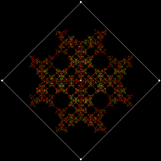
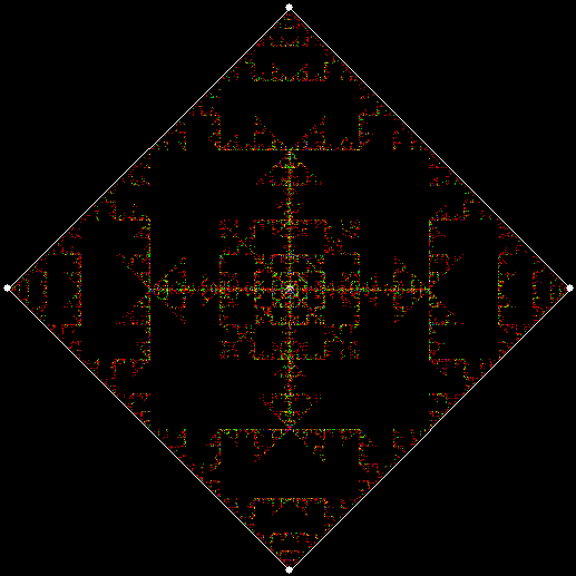
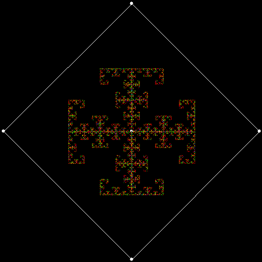
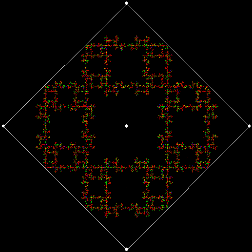
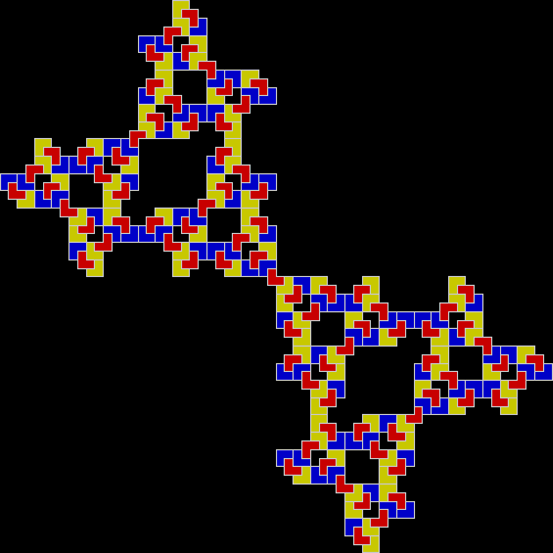
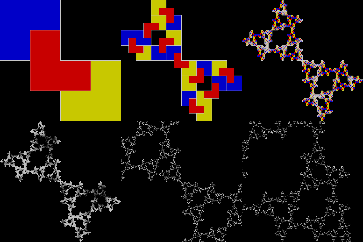
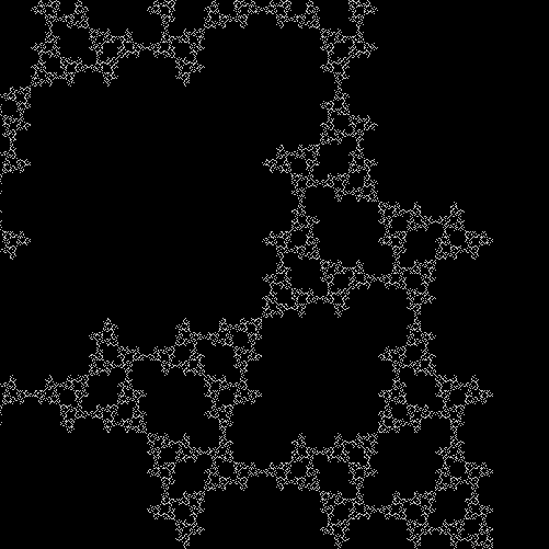
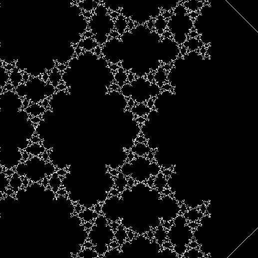
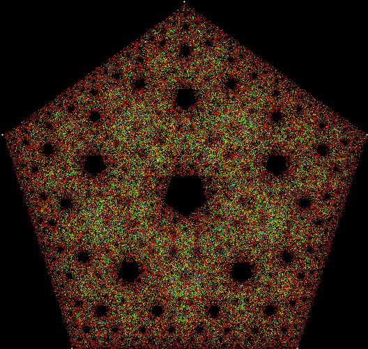
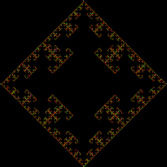
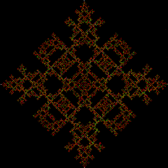
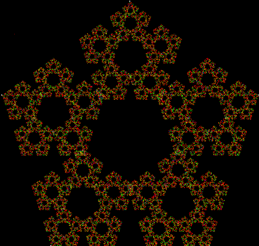
Abstract: The game of chess is the most widely-studied domain in the history of artificial intelligence. The strongest programs are based on a combination of sophisticated search techniques, domain-specific adaptations, and handcrafted evaluation functions that have been refined by human experts over several decades. In contrast, the AlphaGo Zero program recently achieved superhuman performance in the game of Go, by tabula rasa reinforcement learning from games of self-play. In this paper, we generalise this approach into a single AlphaZero algorithm that can achieve, tabula rasa, superhuman performance in many challenging domains. Starting from random play, and given no domain knowledge except the game rules, AlphaZero achieved within 24 hours a superhuman level of play in the games of chess and shogi (Japanese chess) as well as Go, and convincingly defeated a world-champion program in each case. — “Mastering Chess and Shogi by Self-Play with a General Reinforcement Learning Algorithm”, 5/XII/2017.
Tag Archives: Programming
Get Your Prox Off #2
Serendipity is the art of making happy discoveries by accident. I made a mistake writing a program to create fractals and made the happy discovery of an attractive new fractal. And also of a new version of an attractive fractal I had seen before.
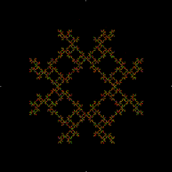
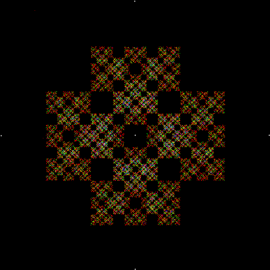
As I described in Get Your Prox Off, you can create a fractal by 1) moving a point towards a randomly chosen vertex of a polygon, but 2) forbidding a move towards the nearest vertex or the second-nearest vertex or third-nearest, and so on. If the polygon is a square, the four possible basic fractals look like this (note that the first fractal is also produced by banning a move towards a vertex that was chosen in the previous move):
v = 4, ban = prox(1)
(ban move towards nearest vertex)
v = 4, ban = prox(2)
(ban move towards second-nearest vertex)
v = 4, ban = prox(3)
v = 4, ban = prox(4)
This program has to calculate what might be called the order of proximity: that is, it creates an array of distances to each vertex, then sorts the array by increasing distance. I was using a bubble-sort, but made a mistake so that the program ran through the array only once and didn’t complete the sort. If this happens, the fractals look like this (note that vertex 1 is on the right, with vertex 2, 3 and 4 clockwise from it):

v = 4, ban = prox(1), sweep = 1
v = 4, ban = prox(2), sweep = 1
v = 4, ban = prox(3), sweep = 1
(Animated version of v4, ban(prox(3)), sw=1)
v = 4, ban = prox(4), sweep = 1
Note that in the last case, where ban = prox(4), a bubble-sort needs only one sweep to identify the most distant vertex, so the fractal looks the same as it does with a complete bubble-sort.
These new fractals looked interesting, so I had the idea of adjusting the number of sweeps in the incomplete bubble-sort: one sweep or two or three and so on (with enough sweeps, the bubble-sort becomes complete, but more sweeps are needed to complete a sort as the number of vertices increases). If there are two sweeps, then ban(prox(1)) and ban(prox(2)) look like this:
v = 4, ban = prox(1), sweep = 2
v = 4, ban = prox(2), sweep = 2
But the fractals produced by sweep = 2 for ban(prox(3)) and ban(prox(4)) are identical to the fractals produced by a complete bubble sort. Now, suppose you add a central point to the polygon and treat that as an additional vertex. If the bubble-sort is incomplete, a ban(prox(1)) fractal with a central point looks like this:
v = 4+c, ban = prox(1), sw = 1
v = 4+c, ban = prox(1), sw = 2
When sweep = 3, an attractive new fractal appears:
v = 4+c, ban = prox(1), sw = 3
v = 4+c, ban = prox(1), sw = 3 (animated)
If you ban two vertices, the nearest and second-nearest, i.e. ban(prox(1), prox(2)), a complete bubble-sort produces a familiar fractal:
v = 4+c, ban = prox(1), prox(2)
And here is ban(prox(2), prox(4)), with a complete bubble-sort:
v = 4, ban = prox(2), prox(4)
If the bubble-sort is incomplete, sweep = 1 and sweep = 2 produce these fractals for ban(prox(1), prox(2)):
v = 4, ban = prox(1), prox(2), sw = 1
v = 4, ban = prox(1), prox(2), sw = 2*
*The second of those fractals is identical to v = 4, ban(prox(2), prox(3)) with a complete bubble-sort.
Here is ban(prox(1), prox(5)) with a complete bubble-sort:
v = 4, ban = prox(1), prox(5)
Now try ban(prox(1), prox(5)) with an incomplete bubble-sort:
v = 4, ban = prox(1), prox(5), sw = 1
v = 4, ban = prox(1), prox(5), sw = 2
When sweep = 3, the fractal I had seen before appears:
v = 4, ban = prox(1), prox(5), sw = 3
v = 4, ban = prox(1), prox(5), sw = 3 (animated)
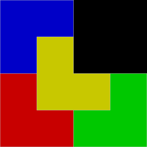
Where had I seen it before? While investigating this rep-tile (a shape that can be tiled with smaller versions of itself):
L-triomino rep-tile
L-triomino rep-tile (animated)
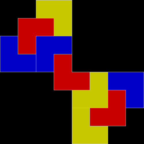
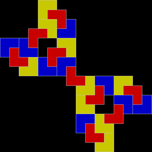
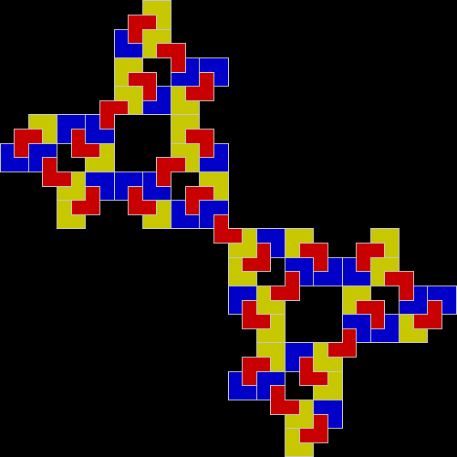
The rep-tile is technically called an L-triomino, because it looks like a capital L and is one of the two distinct shapes you can create by joining three squares at the edges. You can create fractals from an L-triomino by dividing it into four copies, discarding one of the copies, then repeating the divide-and-discard at smaller and smaller scales:
L-triomino fractal stage #1
L-triomino fractal stage #2
L-triomino fractal stage #3
L-triomino fractal stage #4
L-triomino fractal stage #5
L-triomino fractal (animated)
L-triomino fractal (close-up)
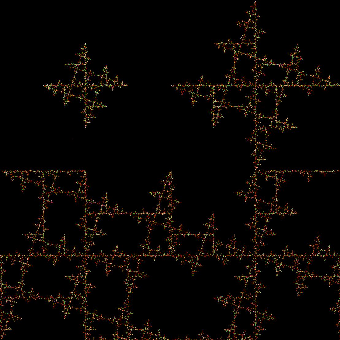
And here’s part of the ban(prox(1), prox(5)) fractal for comparison:
So you can get to the same fractal (or versions of it), by two apparently different routes: random movement of a point inside a square or repeatedly dividing-and-discarding the sub-copies of an L-triomino. That’s serendipity!
Previously pre-posted:
V for Vertex
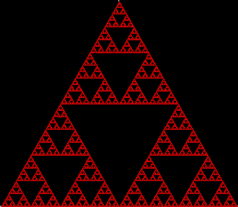
To create a simple fractal, take an equilateral triangle and divide it into four more equilateral triangles. Remove the middle triangle. Repeat the process with each new triangle and go on repeating it. You’ll end up with a shape like this, which is known as the Sierpiński triangle, after the Polish mathematician Wacław Sierpiński (1882-1969):
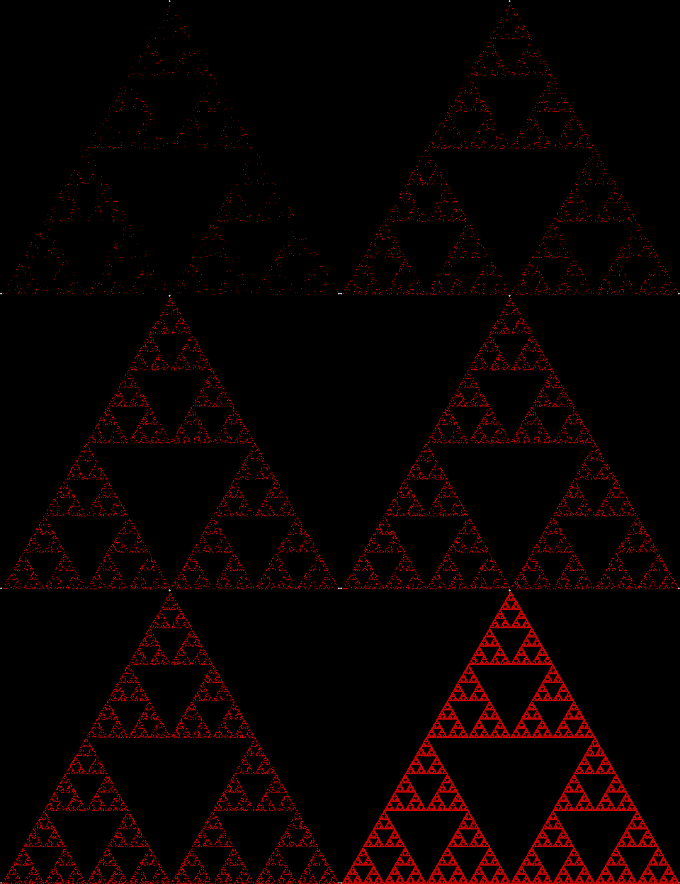
But you can also create the Sierpiński triangle one pixel at a time. Choose any point inside an equilateral triangle. Pick a corner of the triangle at random and move half-way towards it. Mark this spot. Then pick a corner at random again and move half-way towards the corner. And repeat. The result looks like this:
A simple program to create the fractal looks like this:
initial()
repeat
fractal()
altervariables()
until falsefunction initial()
v = 3 [v for vertex]
r = 500
lm = 0.5
endfuncfunction fractal()
th = 2 * pi / v
[the following loop creates the corners of the triangle]
for l = 1 to v
x[l]=xcenter + sin(l*th) * r
y[l]=ycenter + cos(l*th) * r
next l
fx = xcenter
fy = ycenter
repeat
rv = random(v)
fx = fx + (x[rv]-fx) * lm
fy = fy + (y[rv]-fy) * lm
plot(fx,fy)
until keypressed
endfuncfunction altervariables()
[change v, lm, r etc]
endfunc
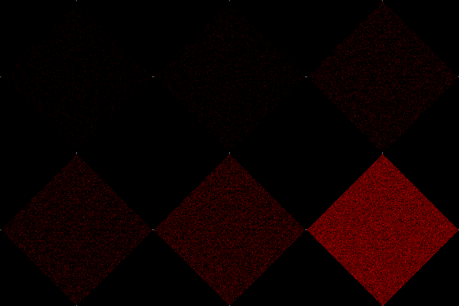
In this case, more is less. When v = 4 and the shape is a square, there is no fractal and plot(fx,fy) covers the entire square.
When v = 5 and the shape is a pentagon, this fractal appears:
But v = 4 produces a fractal if a simple change is made in the program. This time, a corner cannot be chosen twice in a row:
function initial()
v = 4
r = 500
lm = 0.5
ci = 1 [i.e, number of iterations since corner previously chosen]
endfuncfunction fractal()
th = 2 * pi / v
for l = 1 to v
x[l]=xcenter + sin(l*th) * r
y[l]=ycenter + cos(l*th) * r
chosen[l]=0
next l
fx = xcenter
fy = ycenter
repeat
repeat
rv = random(v)
until chosen[rv]=0
for l = 1 to v
if chosen[l]>0 then chosen[l] = chosen[l]-1
next l
chosen[rv] = ci
fx = fx + (x[rv]-fx) * lm
fy = fy + (y[rv]-fy) * lm
plot(fx,fy)
until keypressed
endfunc
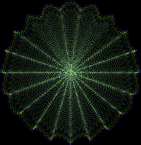
One can also disallow a corner if the corner next to it has been chosen previously, adjust the size of the movement towards the chosen corner, add a central point to the polygon, and so on. Here are more fractals created with such variations: