Serendipity is the art of making happy discoveries by accident. I made a mistake writing a program to create fractals and made the happy discovery of an attractive new fractal. And also of a new version of an attractive fractal I had seen before.
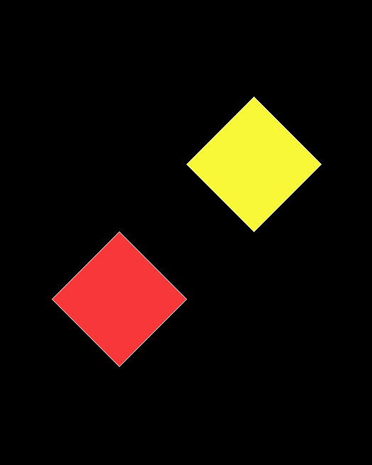
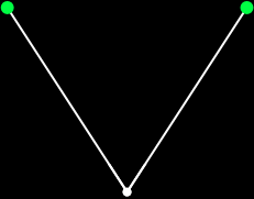
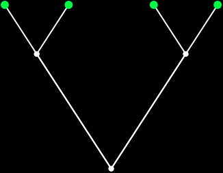
As I described in Get Your Prox Off, you can create a fractal by 1) moving a point towards a randomly chosen vertex of a polygon, but 2) forbidding a move towards the nearest vertex or the second-nearest vertex or third-nearest, and so on. If the polygon is a square, the four possible basic fractals look like this (note that the first fractal is also produced by banning a move towards a vertex that was chosen in the previous move):

v = 4, ban = prox(1)
(ban move towards nearest vertex)

v = 4, ban = prox(2)
(ban move towards second-nearest vertex)

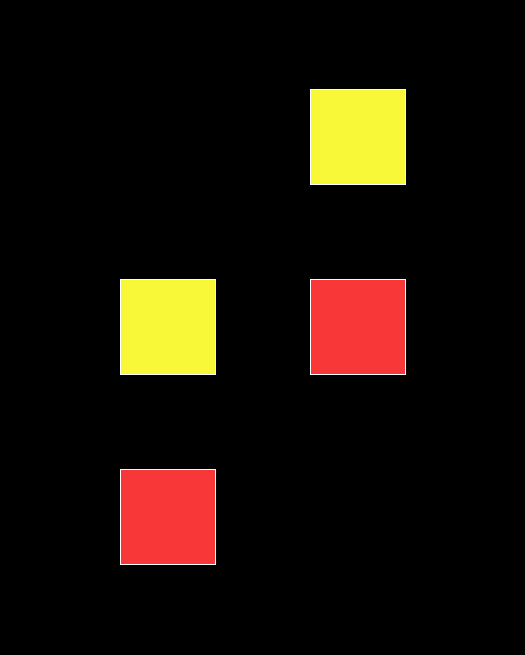
v = 4, ban = prox(3)

v = 4, ban = prox(4)
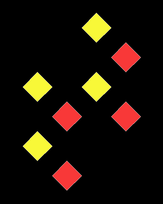
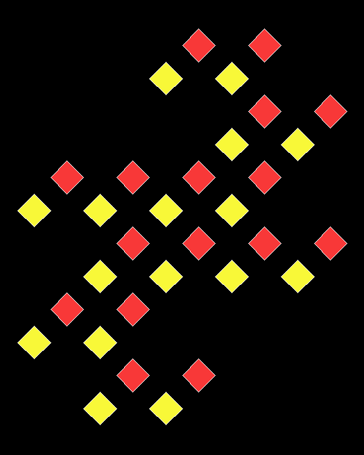
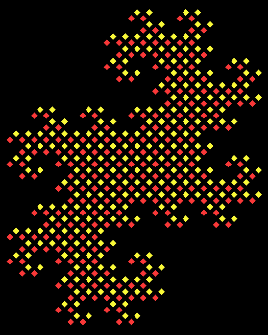
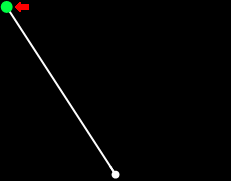
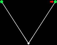
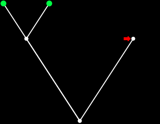
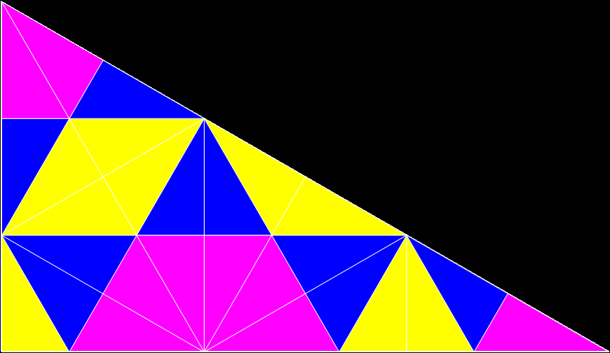
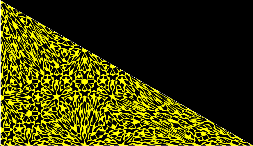
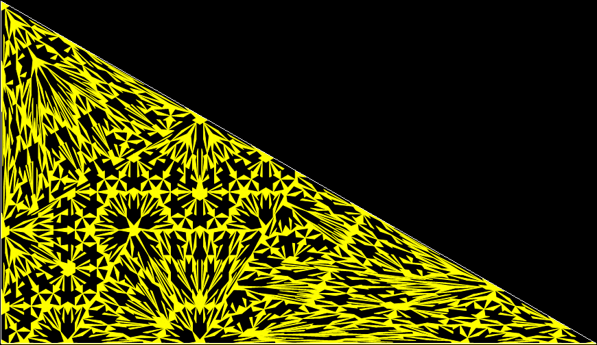
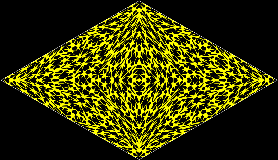
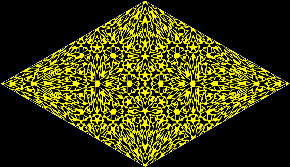
This program has to calculate what might be called the order of proximity: that is, it creates an array of distances to each vertex, then sorts the array by increasing distance. I was using a bubble-sort, but made a mistake so that the program ran through the array only once and didn’t complete the sort. If this happens, the fractals look like this (note that vertex 1 is on the right, with vertex 2, 3 and 4 clockwise from it):
v = 4, ban = prox(1), sweep = 1

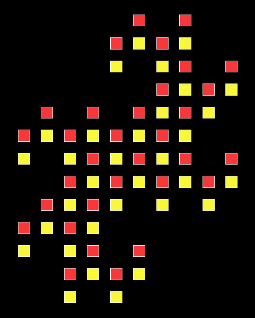
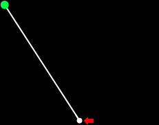
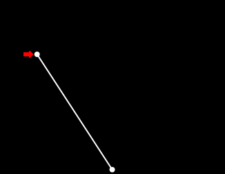
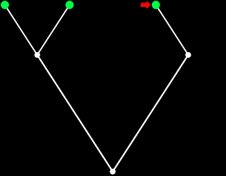
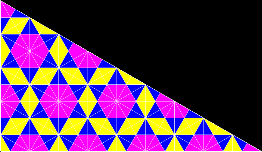
v = 4, ban = prox(2), sweep = 1
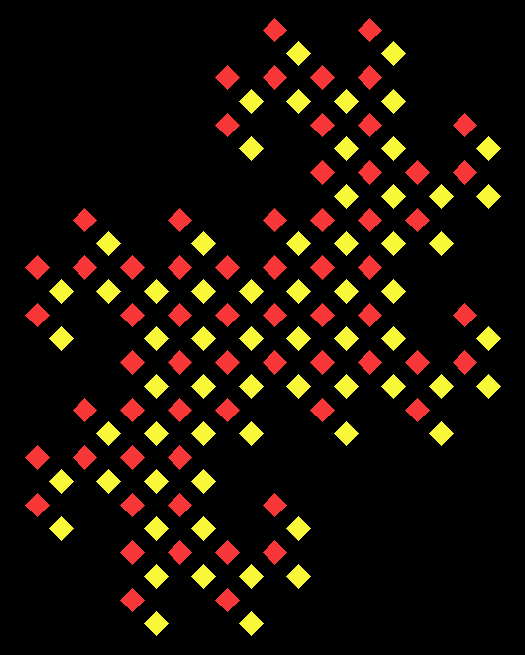
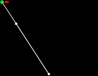
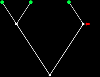
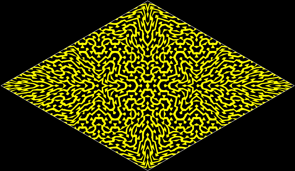
v = 4, ban = prox(3), sweep = 1
(Animated version of v4, ban(prox(3)), sw=1)

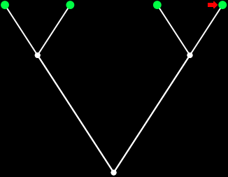
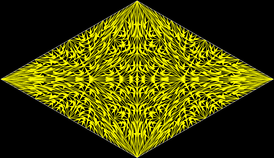
v = 4, ban = prox(4), sweep = 1
Note that in the last case, where ban = prox(4), a bubble-sort needs only one sweep to identify the most distant vertex, so the fractal looks the same as it does with a complete bubble-sort.
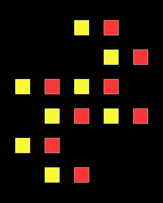
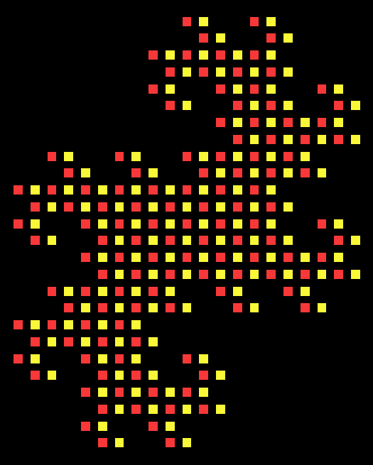
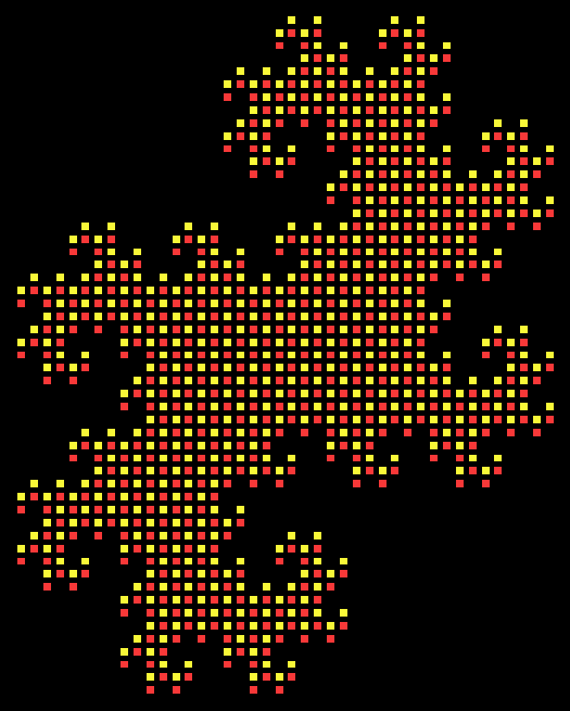
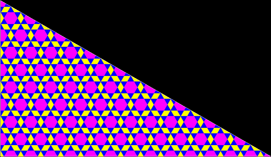
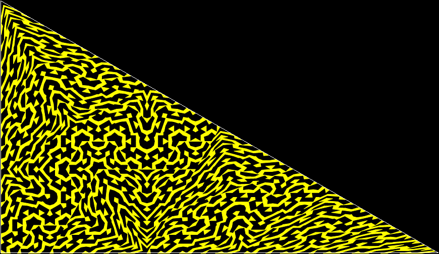
These new fractals looked interesting, so I had the idea of adjusting the number of sweeps in the incomplete bubble-sort: one sweep or two or three and so on (with enough sweeps, the bubble-sort becomes complete, but more sweeps are needed to complete a sort as the number of vertices increases). If there are two sweeps, then ban(prox(1)) and ban(prox(2)) look like this:
v = 4, ban = prox(1), sweep = 2
v = 4, ban = prox(2), sweep = 2
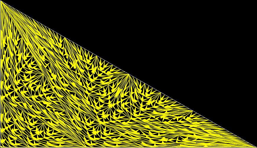
But the fractals produced by sweep = 2 for ban(prox(3)) and ban(prox(4)) are identical to the fractals produced by a complete bubble sort. Now, suppose you add a central point to the polygon and treat that as an additional vertex. If the bubble-sort is incomplete, a ban(prox(1)) fractal with a central point looks like this:
v = 4+c, ban = prox(1), sw = 1
v = 4+c, ban = prox(1), sw = 2
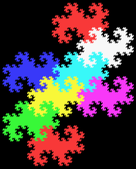
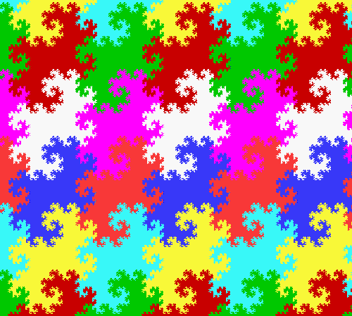
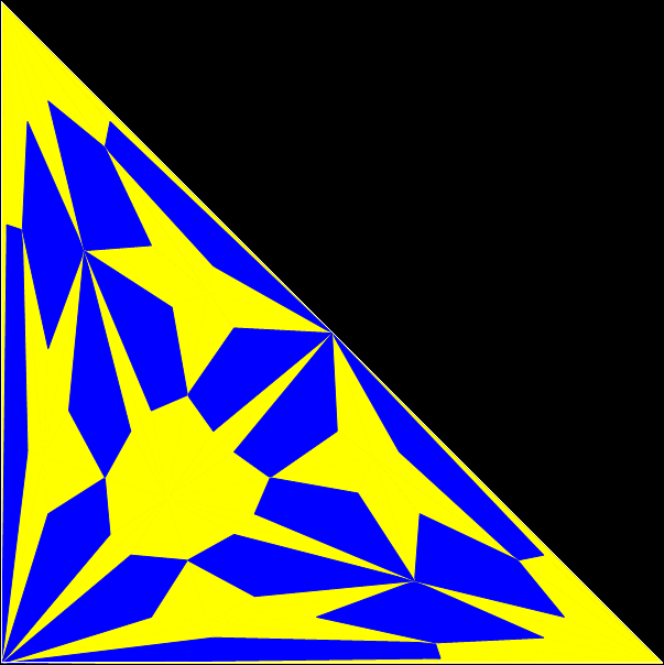
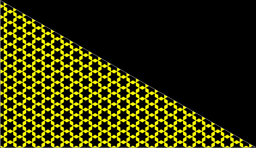
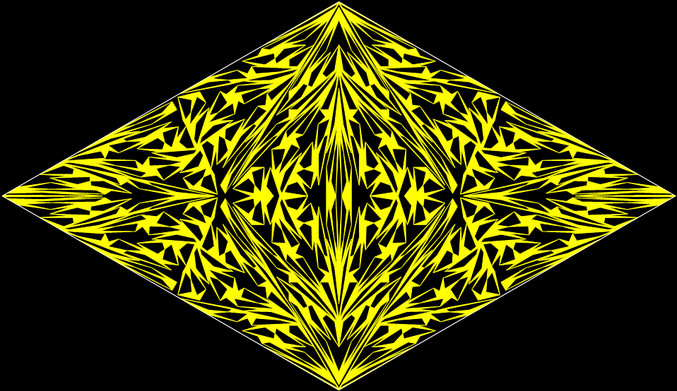
When sweep = 3, an attractive new fractal appears:
v = 4+c, ban = prox(1), sw = 3

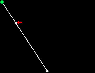
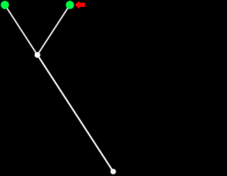
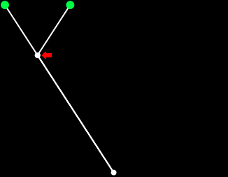
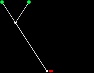
v = 4+c, ban = prox(1), sw = 3 (animated)
If you ban two vertices, the nearest and second-nearest, i.e. ban(prox(1), prox(2)), a complete bubble-sort produces a familiar fractal:

v = 4+c, ban = prox(1), prox(2)
And here is ban(prox(2), prox(4)), with a complete bubble-sort:
v = 4, ban = prox(2), prox(4)
If the bubble-sort is incomplete, sweep = 1 and sweep = 2 produce these fractals for ban(prox(1), prox(2)):

v = 4, ban = prox(1), prox(2), sw = 1

v = 4, ban = prox(1), prox(2), sw = 2*
*The second of those fractals is identical to v = 4, ban(prox(2), prox(3)) with a complete bubble-sort.
Here is ban(prox(1), prox(5)) with a complete bubble-sort:
v = 4, ban = prox(1), prox(5)
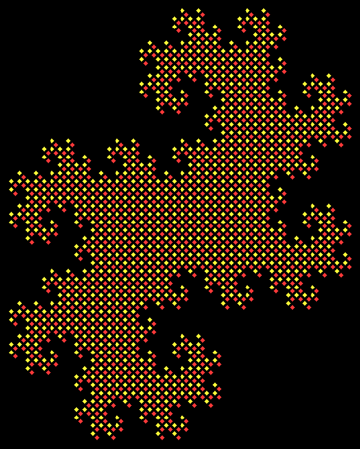
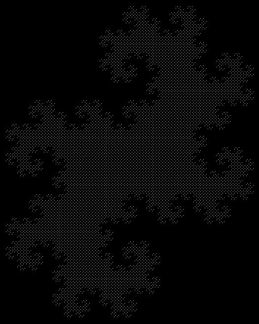
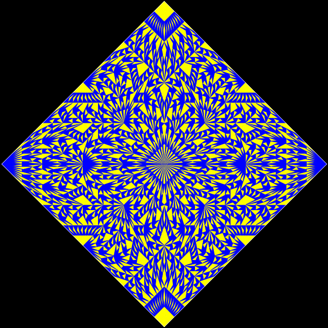
Now try ban(prox(1), prox(5)) with an incomplete bubble-sort:

v = 4, ban = prox(1), prox(5), sw = 1

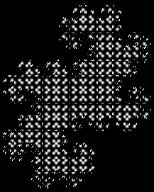
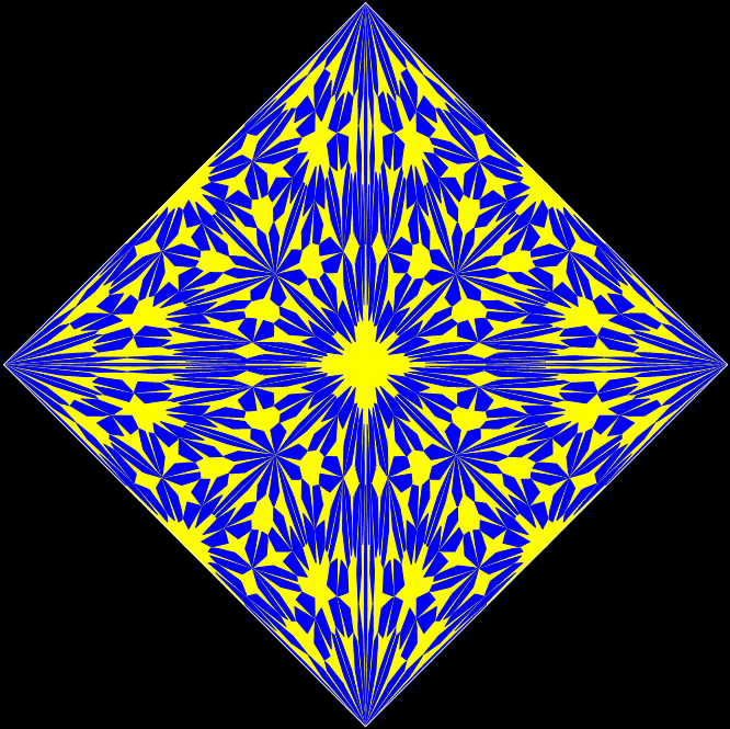
v = 4, ban = prox(1), prox(5), sw = 2
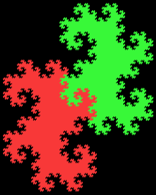
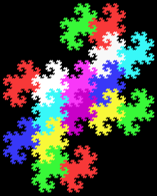
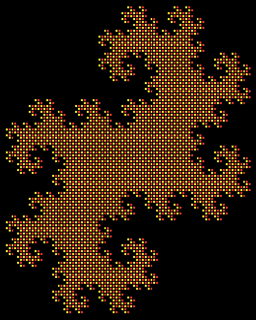
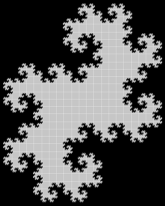
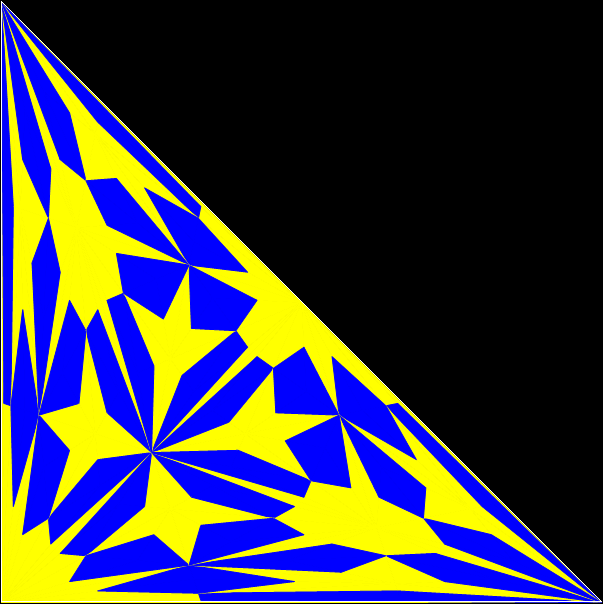
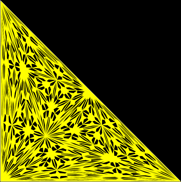
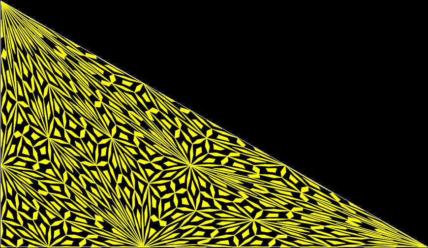
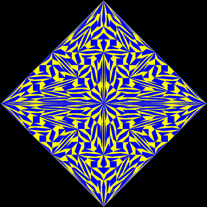
When sweep = 3, the fractal I had seen before appears:

v = 4, ban = prox(1), prox(5), sw = 3

v = 4, ban = prox(1), prox(5), sw = 3 (animated)
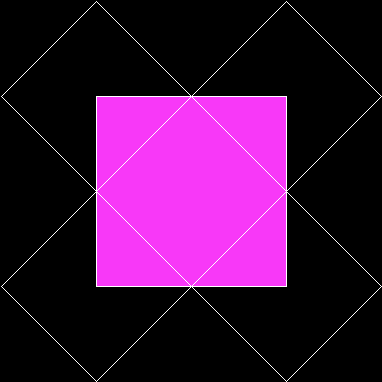
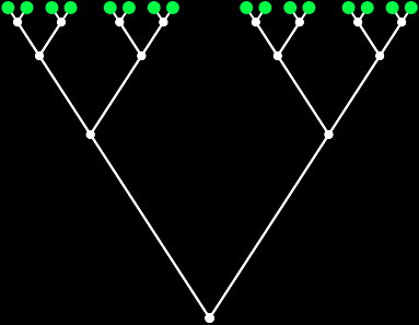
Where had I seen it before? While investigating this rep-tile (a shape that can be tiled with smaller versions of itself):

L-triomino rep-tile

L-triomino rep-tile (animated)
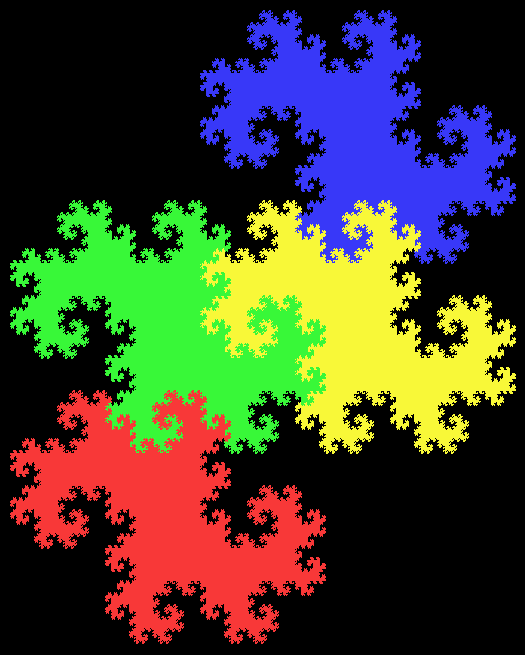
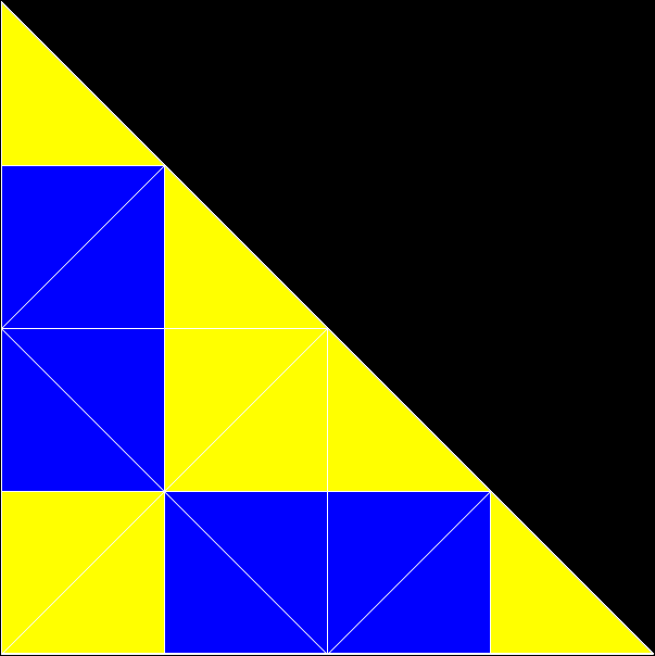
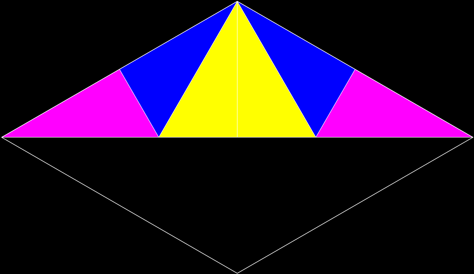
The rep-tile is technically called an L-triomino, because it looks like a capital L and is one of the two distinct shapes you can create by joining three squares at the edges. You can create fractals from an L-triomino by dividing it into four copies, discarding one of the copies, then repeating the divide-and-discard at smaller and smaller scales:

L-triomino fractal stage #1
L-triomino fractal stage #2

L-triomino fractal stage #3
L-triomino fractal stage #4
L-triomino fractal stage #5
L-triomino fractal (animated)
L-triomino fractal (close-up)
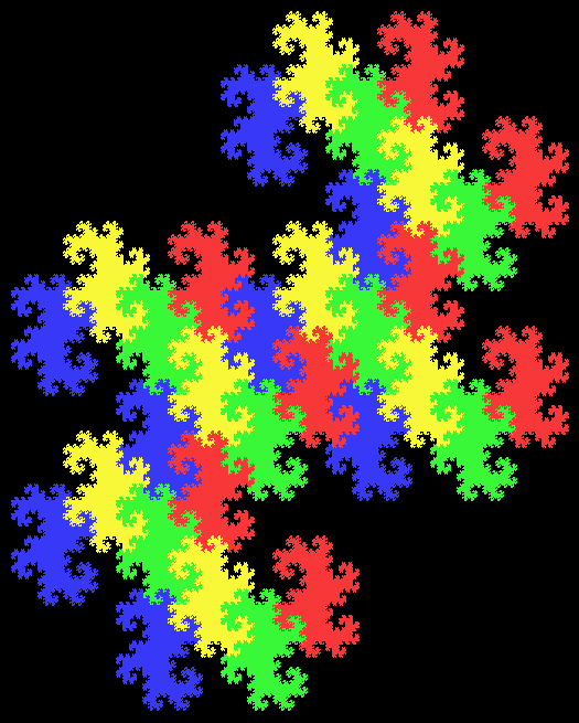
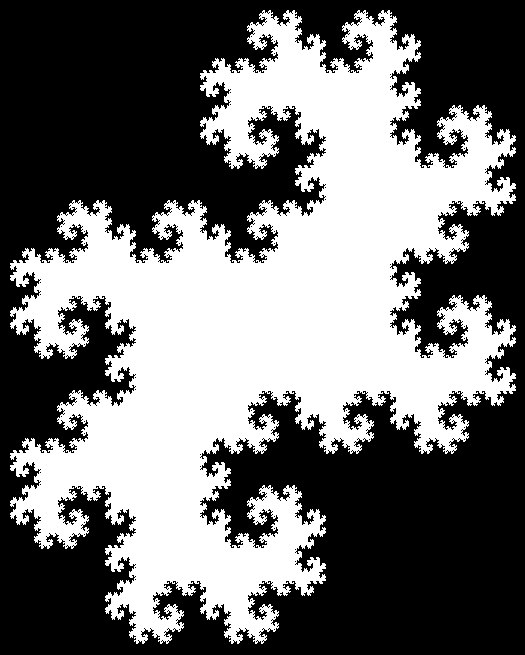
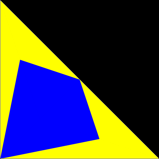
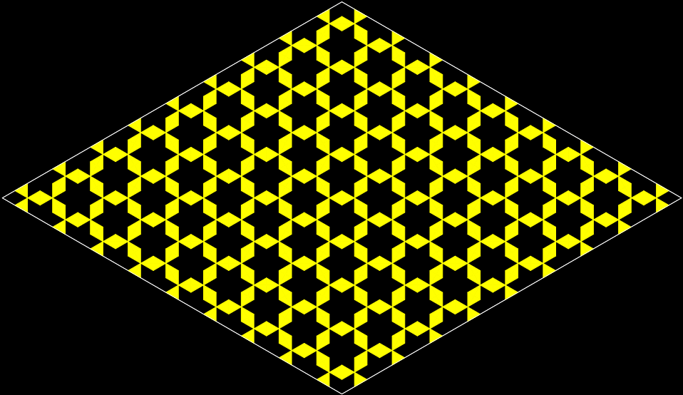
And here’s part of the ban(prox(1), prox(5)) fractal for comparison:

So you can get to the same fractal (or versions of it), by two apparently different routes: random movement of a point inside a square or repeatedly dividing-and-discarding the sub-copies of an L-triomino. That’s serendipity!
Previously pre-posted:
• Get Your Prox Off