Scout the Routes

Triangles? Yes. Squares? No. If you scout the routes with a triangle, you get a beautiful fractal. If you scout the routes with a square, you don’t. Here’s what you get with a triangle:

A Sierpiński triangle


But how do you scout the routes? (That phrase works best in the American dialects where “scout” rhymes with “route”.) Simple: you mark the final positions reached when a point traces all possible ways of jumping, say, eight times 1/2-way towards the vertices of a polygon. Here’s an animation of a point scouting the routes of eight jumps towards the vertices of a triangle (it starts each time at the center):

Creating a Sierpiński triangle by scouting the routes (animated at Ezgif)


If you scout the routes with a square, you don’t get a fractal. Instead, the interior of the square fills evenly (and boringly) with the end-points of the routes:

Scouting the routes with a square (animated at Ezgif)


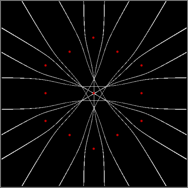
But you can create fractals with a square if you out routes as you scout routes. That is, if you exclude some routes and don’t mark their end-points. One way to do this is to compare the proposed next jump-vertex (vertex-jumped-towards) with the previous jump-vertex. For example, if the proposed jump-vertex, jv[t], is the same as the previous jump-vertex, jv[t-1], you don’t jump towards jv[t] or you jump towards it in a different way. The test is jv[t] = jv[t-1] + vi. If vi = 0 and you jump towards the clockwise neighbor of jv when the test is true, you get a fractal looking like this:

vi = 0, action = jv → jv + 1


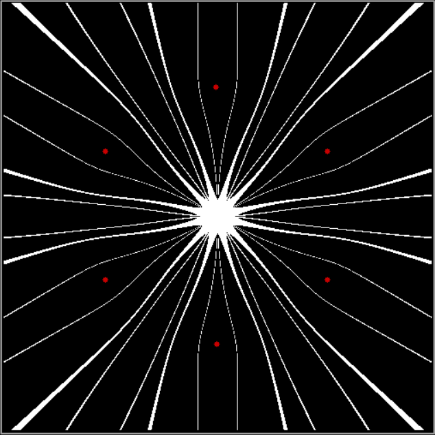
Here’s the fractal if you jump towards the clockwise-neighbor-but-one when the test is true:

vi = 0, action = jv + 2


Now try varying the vi of the jv[t-1] + vi:

vi = 2, action = jv + 2


vi = 2, action = jv + 1


vi = 3, action = jv + 1


Or what about jumping in a different way towards jv when the test is true? If you jump 2/3 of the way rather 1/2, you get his fractal:

vi = 2, action = jump 2/3


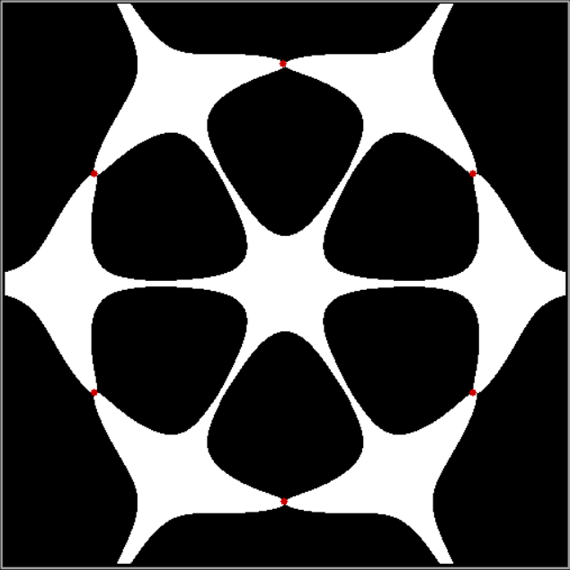
And if you jump 4/3 of the way (i.e., you overshoot the vertex jv), you get this fractal:

vi = 0, action = jump 4/3rds to vertex


vi = 0, jump 4/3 (guide-square removed)


vi = 2, jump 4/3rds (guide-square removed)


And in this fractal the point jumps 2/3 of the way to the center of the square when the test is true:

vi = 2, action = jump 2/3rds of way to center of square


But why apply only one test to jv[1] and use only when one alternative jump? If jv[t] = jv[t-1] + 1 or jv[t] = jv[t-1] + 3, jv[t] becomes jv[t]+1 or jv[t]+3, respectively, you get this fractal:

vi = 1, jv + 1; vi = 3, jv + 3


Here are more fractals created by single and double tests:

vi = 1, jv + 1


vi = 0, jump 2/3


vi = 0, jump towards center 2/3rds


vi = 1, jump-center 2/3


vi = 2, jump 1/3; vi = 3, jump 1/1 (i.e, 1)


vi = 0, jv + 2; vi = 2, jump-center 1/2


vi = 0, jv + 2; vi = 2, jump-center 2/3


vi = 0, jv + 2; vi = 2, jump-center 4/3


vi = 0, jv + 1; vi = 2, jump 2/3


vi = 0, jv + 2; vi = 2, jump 2/3


vi = 0, jump 4/3; vi = 2, jv + 2


vi = 0, jump 2/3; vi = 2, jv + 1


vi = 0, jump 4/3; vi = 1, jv + 2


vi = 0, jump 2/3; vi = 2, jump 1/3


vi =0, jump 1/3; vi = 2, jump 2/3


vi = 0, jump 0/1 (i.e, 0); vi = 2, jump 1/3


Lime Time

What do you get if you list every successive pair of entries in this sequence?

1, 2, 1, 3, 2, 3, 1, 4, 3, 4, 1, 5, 2, 5, 3, 5, 4, 5, 1, 6, 5, 6, 1, 7, 2, 7, 3, 7, 4, 7, 5, 7, 6, 7, 1, 8, 3, 8, 5, 8, 7, 8, 1, 9, 2, 9, 4, 9, 5, 9, 7, 9, 8, 9, 1, 10, 3, 10, 7, 10, 9, 10, 1, 11, 2, 11, 3, 11, 4, 11, 5, 11, 6, 11, 7, 11, 8, 11, 9, 11, 10, 11, 1, 12, 5, 12, 7, 12, 11, 12, 1, 13, … — A038568 at the Online Encyclopedia of Integer Sequence

You get the rational fractions ordered by denominator in their simplest form: 1/2, 1/3, 2/3, 1/4, 3/4, 1/5, 2/5, 3/5… There are no pairs like 2/4 and 5/35, because those can be simplified: 2/4 → 1/2; 15/35 → 3/7. You can get the same set of rational fractions by listing every successive pair in this sequence, the Stern-Brocot sequence:

1, 2, 1, 3, 2, 3, 1, 4, 3, 5, 2, 5, 3, 4, 1, 5, 4, 7, 3, 8, 5, 7, 2, 7, 5, 8, 3, 7, 4, 5, 1, 6, 5, 9, 4, 11, 7, 10, 3, 11, 8, 13, 5, 12, 7, 9, 2, 9, 7, 12, 5, 13, 8, 11, 3, 10, 7, 11, 4, 9, 5, 6, 1, 7, 6, 11, 5, 14, 9, 13, 4, 15, 11, 18, 7, 17, 10, 13, 3, 14, 11, 19, 8, 21, 13, 18, 5, 17, 12, 19, … — A002487 at the OEIS

But the fractions don’t come ordered by denominator this time. In fact, they seem to come at random: 1/2, 1/3, 2/3, 1/4, 3/5, 2/5, 3/4, 1/5, 4/7, 3/8, 5/7, 2/7, 5/8… But they’re not random at all. There’s a complicated way of generating them and a simple way. An amazingly simple way, I think:

Moshe Newman proved that the fraction a(n+1)/a(n+2) can be generated from the previous fraction a(n)/a(n+1) = x by 1/(2*floor(x) + 1 – x). The successor function f(x) = 1/(floor(x) + 1 – frac(x)) can also be used. — A002487, “Stern-Brocot Sequence”, at the OEIS

In another form, the Stern-Brocot sequence is generated by what’s called the Calkin-Wilf Tree. Now suppose you use the Stern-Brocot sequence to supply the x co-ordinate of an L-graph whose arms run from 0 to 1. And you use the Calkin-Wilf Tree to supply the y co-ordinate of the L-tree. What do you get? As I described in “I Like Gryke”, you get this fractal:

Limestone fractal


I call it a limestone fractal or pavement fractal or gryke fractal, because it reminds me of the fissured patterns you see in the limestone pavements of the Yorkshire Dales:

Fissured limestone pavement, Yorkshire Dales (Wikipedia)


But what happens when you plot the (x,y) of the Stern-Brocot sequence and the Calkin-Wilf Tree on a circle instead? You get an interestingly distorted limestone fractal:

Limestone fractal on circle


You can also plot the (x,y) around the perimeter of a polygon, then stretch the polygon into a circle. Here’s a square:

Limestone fractal on square

Limestone square stretched to circle


And here are a pentagon, hexagon, heptagon and octagon — note the interesting perspective effects:

Limestone fractal on pentagon

Limestone pentagon stretched to circle


Limestone fractal on hexagon

Limestone hexagon stretched to circle


Limestone fractal on heptagon

Limestone heptagon stretched to circle


Limestone fractal on octagon

Limestone octagon stretched to circle


And finally, here are animations of limestone polygons stretching to circles:

Limestone square stretched to circle (animated at EZgif)


Limestone pentagon to circle (animated)


Limestone hexagon to circle (animated)


Limestone heptagon to circle (animated)


Limestone octagon to circle (animated)


Previously Pre-Posted (Please Peruse)

I Like Gryke — a first look at the limestone fractal

Punctuated Pairimeters

Imagine using the digits of n in two different bases to generate two fractions, a/b and c/d, where a/b < 1 and c/d < 1 (see Appendix for a sample program). Now use the fractions to find a pair of points on the perimeter of a circle, (x1, y1) and (x2, y2), then calculate and mark the midpoint of (x1, y1) and (x2, y2). If the bases have a prime factor in common, pretty patterns will appear from this punctuated pairimetry:

b1 = 2; b2 = 6


b1 = 2; b2 = 10


b1 = 2; b2 = 14


b1 = 4; b2 = 10


b1 = 4; b2 = 20


b1 = 4; b2 = 28


b1 = 6; b2 = 42


b1 = 12; b2 = 39


b1 = 24; b2 = 28


b1 = 28; b2 = 40


b1 = 32; b2 = 36


b1 = 42; b2 = 78


Appendix: Sample Program for Pairimetry

GetXY(xyi)=

fr = 0
recip = 1
bs = base[xyi]
for gi = 1 to di[xyi]
recip = recip/bs
fr += d[xyi,gi] * recip
next gi

x[xyi] = xcenter + sin(pi2 * fr) * radius
y[xyi] = ycenter + cos(pi2 * fr) * radius

endproc

Dinc(i1) =

d[i1,1]++;
if d[i1,1] == base[i1] then

i2 = 1

while d[i1,i2] == base[i1]

d[i1,i2] = 0
i2++;
d[i1,i2]++;

endwhile

if i2 > di[i1] then di[i1] = i2 endif

endif

endproc

Drawfigure =

base = x = y = di = array(2)
d = array(2,100)
radius = 100
pi2 = pi * 2
base[1] = 2
base[2] = 6
di[1] = 1
di[2] = 1

while true

for i = 1 to 2
call Dinc(i)
call GetXY(i)
next i

plot (x[1]+x[2]) / 2, (y[1] + y[2]) / 2

endwhile

endproc

call drawfigure

Partitional Pulchritude

If you want a good example of how, in math, something very simple can quickly get very deep, just look at partitions. Here are the partitions of 1 to 5, that is, the ways 1 to 5 can be expressed as a sum of integers smaller than or equal to themselves:

1 = 1

numbpart(1) = 1


2 = 2
1 + 1 = 2

numbpart(2) = 2


3 = 3
1 + 2 = 3
1 + 1 + 1 = 3

numbpart(3) = 3


4 = 4
1 + 3 = 4
2 + 2 = 4
1 + 1 + 2 = 4
1 + 1 + 1 + 1 = 4

numbpart(4) = 5


5 = 5
1 + 4 = 5
2 + 3 = 5
1 + 1 + 3 = 5
1 + 2 + 2 = 5
1 + 1 + 1 + 2 = 5
1 + 1 + 1 + 1 + 1 = 5

numbpart(5) = 7


It’s very easy to understand the concept of partitions, but very difficult to understand how partitions behave. For example, here is numbpart(n), the count of partitions for 1, 2, 3,…

1, 2, 3, 5, 7, 11, 15, 22, 30, 42, 56, 77, 101, 135, 176, 231, 297, 385, 490, 627, 792, 1002, 1255, 1575, 1958, 2436, 3010, 3718, 4565, 5604, 6842, 8349, 10143, 12310, 14883, 17977, 21637, 26015, 31185, 37338, 44583, 53174, 63261, 75175, 89134, 105558, 124754, 147273, 173525, 204226, … A000041 at the Online Encyclopedia of Integer Sequences, “a(n) is the number of partitions of n (the partition numbers)”

What’s the formula for numbpart(n)? That’s a tricky question. And what’s the formula for the curves produced by counting the various lengths of partitions(n)? That’s another tricky question, but one thing is easy to see. As n gets bigger, the graph of countlen(partitions(n)) acquires a strange, lopsided beauty. Here are the partitions of 8, with the count of how many partitions of a particular length there are:

8 = 8 (1 partition of length 1)
1 + 7 = 8
2 + 6 = 8
3 + 5 = 8
4 + 4 = 8 (4 partitions of length 2)
1 + 1 + 6 = 8
1 + 2 + 5 = 8
1 + 3 + 4 = 8
2 + 2 + 4 = 8
2 + 3 + 3 = 8 (5 of length 3)
1 + 1 + 1 + 5 = 8
1 + 1 + 2 + 4 = 8
1 + 1 + 3 + 3 = 8
1 + 2 + 2 + 3 = 8
2 + 2 + 2 + 2 = 8 (5 of length 4)
1 + 1 + 1 + 1 + 4 = 8
1 + 1 + 1 + 2 + 3 = 8
1 + 1 + 2 + 2 + 2 = 8 (3 of length 5)
1 + 1 + 1 + 1 + 1 + 3 = 8
1 + 1 + 1 + 1 + 2 + 2 = 8 (2 of length 6)
1 + 1 + 1 + 1 + 1 + 1 + 2 = 8 (1 of length 7)
1 + 1 + 1 + 1 + 1 + 1 + 1 + 1 = 8 (1 of length 8)

When counts like that are shown as a graph, the graphs look like this (maximum counts are normalized to the same height):


graph of countlen(partitions(2))


countlen(partitions(3))


countlen(partitions(4))


countlen(partitions(5))


countlen(partitions(6))


countlen(partitions(7))


countlen(partitions(8))


countlen(partitions(9))


countlen(partitions(10))


countlen(partitions(15))


countlen(partitions(20))


countlen(partitions(30))


countlen(partitions(40))


countlen(partitions(50))


countlen(partitions(60))


countlen(partitions(70))


countlen(partitions(80))


countlen(partitions(90))


countlen(partitions(100))


Animated gif of partlen graphs (courtesy EZgif)


The graphs have a long, low right tail because the counts rise to great heights very quick, then fall away again, as you can see with partitions(100):

1 = count(partitions(10),len=1)
50 = count(partitions(10),len=2)
833 = count(partitions(10),len=3)
7153 = count(partitions(10),len=4)
38225 = count(partitions(10),len=5)
143247 = count(partitions(10),len=6)

[…]

10643083 = count(partitions(10),len=16)
11022546 = count(partitions(10),len=17)
11087828 = count(partitions(10),len=18)
10885999 = count(partitions(10),len=19)
10474462 = count(partitions(10),len=20)

[…]

30 = count(partitions(10),len=91)
22 = count(partitions(10),len=92)
15 = count(partitions(10),len=93)
11 = count(partitions(10),len=94)
7 = count(partitions(10),len=95)
5 = count(partitions(10),len=96)
3 = count(partitions(10),len=97)
2 = count(partitions(10),len=98)
1 = count(partitions(10),len=99)
1 = count(partitions(10),len=100)

Sorted for D’s nand Wizz

As I’ve pre-previously pointed out, there are an infinite number of points in the plane. And in part of the plane. So you have to pare points to create interesting shapes. One way of paring points is by comparing them. After you’ve compared them, you can sort them. For example, you can compare the distance from (x,y) to the four vertices of a square. Then you can sort the distances from nearest to furthest. Then you can mark (x,y) if the distance to, say, the nearest vertice from (x,y) is evenly divisible by 2 when measured in pixels or some other unit. When you do that, you might get an image like this (depending on the hardware and software you use):

Distance to nearest vertex is evenly divisible by 2, i.e. d mod 2 = 0 for v1 (vertices marked in red)


Or you can mark (x,y) if the distance to the nearest vertex is a triangular number:

is_triangular(d) for v1


Or a square number:

is_square(d) for v1


Or you can test the distance to the second-nearest vertex:

d mod 2 = 0 for v2


And the third-nearest (or second-furthest) vertex:

d mod 2 = 0 for v3


And furthest vertex:

d mod 2 = 0 for v4


Now try expanding or contracting the square:

d mod 2 = 0 for v1 on square * 2


d mod 2 = 0 for v1 on square * 3


d mod 2 = 0 for v1 on square * 0.5


d mod 2 = 0 for v1 on square * 1.5


d mod 2 = 0 for v1 on square * 5


d mod 2 = 0 for v1 on square * 20


d mod 2 = 0 for v1 on square * 100


Finally, here are some more mandala-like images created by using various d mod m on an expanded square (the images should be horizontally and vertically mirror-symmetrical, but my software introduced artefacts):

d mod 2 = 0 for v1 on square * 200
(open in separate window for better detail)


d mod 3 = 0 for v1 on square * 200


d mod 4 = 0 for v1 on square * 200


d mod 5 = 0 for v1 on square * 200


d mod 6 = 0 for v1 on square * 200


d mod 7 = 0 for p1 on square * 200


d mod 8 = 0 for p1 on square * 200


d mod 9 = 0 for p1 on square * 200


d mod 2..9 = 0 for p1 on square * 200 (animated at EZgif)


Post-Performative Post-Scriptum…

The title of this incendiary intervention is a paronomasia on “Sorted for E’s and Wizz”, a song offa of 1995 album Different Class by Sheffield Brit-popsters Pulp rebelliously referencing counter-cultural consumption of psychoactive drugs ecstasy and amphetamine. My program sorted distances, i.e. d’s, but not wizz, therefore it sorted d’s and-not wizz. In Boolean logic, nand means “and-not” (roughly speaking).


Previously Pre-Posted (Please Peruse)…

Points Pared — an earlier look at points and polygons

I Like Gryke

Sometimes I find fractals. And sometimes fractals find me. Here’s a fractal that found me:

Limestone fractal #1


I call it a limestone fractal or pavement fractal or gryke fractal, because it reminds me of the fissured patterns you see in the limestone pavements of the Yorkshire Dales:

Fissured limestone pavement, Yorkshire Dales (Wikipedia)


The limestone blocks are called clints and the larger fissures between them are called grykes, with kamenitza and karren (from Slavic and German, respectively) for smaller pits and grooves:

Limestone linguistics (Dales Rocks)


Here’s the me-finding fractal again, in a slightly different version:

Limestone fractal #2


How did it find me? Well, I wasn’t looking for fractals, but looking at fractions. Farey fractions and Calkin-Wilf fractions, to be precise. They can both be represented as bifurcating trees, like this:

Calkin-Wilf tree (Wikipedia)


Both trees produce all the irreducible rational fractions — but in a different order. That’s why they create a fractal (rather than a 45° line). By following the same path in both bifurcating trees, I generated parallel sequences of Farey and Calkin-Wilf fractions, then used the Farey fractions to represent x in a 1×1 square and the Calkin-Wilf fractions to represent y (where the Calkin-Wilfs, a/b, were greater than 1, I simply a/b → b/a). When you do that (or use Stern-Brocot fractions instead of the Farey fractions), you get the limestone fractal.

I think it looks better in the second version (which is the one that found me, in fact). For LF #2, I was using standard binary numbers to generate the parallel sequences, so the leftmost digit was always 1 and final step of the tree-search was always in the same direction. Here’s LF #2 as black-on-white rather than white-on-black:

Limestone fractal #2 (black-on-white)


And here is the formation of LF #1 as an animated gif:

Growth of limestone fractal (animated at ezGIF)


And if that’s a me-finding fractal, what about me-found fractals? Here’s one:

The Hourglass Fractal (animated gif optimized at ezGIF)

Hourglass fractal


I can say “I found that fractal” because I was looking for fractals when it appeared on the screen. And re-appeared (and re-re-appeared), because I’ve found it using different methods.


Elsewhere Other-Accessible

Hour Power — more on the hourglass fractal

The Bellissima Curve

The bell curve is a shape that appears when you make a graph by counting all possible sums of a range of integers like 1, 2, 3, 4, 5, 6, 7, 8, 9, 10. The smallest sum you can get is 1; the largest is 55 = 1 + 2 + 3 + 4 + 5 + 6 + 7 + 8 + 9 + 10. But there’s only one sum of 1 and only one sum of 55. Other sums are more common:

• 10 = 1 + 2 + 3 + 4
• 10 = 1 + 2 + 7
• 10 = 1 + 3 + 6
• 10 = 1 + 4 + 5
• 10 = 2 + 3 + 5
• 10 = 2 + 8
• 10 = 3 + 7
• 10 = 4 + 6
• 10 = 10

So there are nine sums of 10. If you graph count-sums with a bigger set of consecutive integers from 1, 2, 3…, you get this shape:

Bell curve from sum-counts with 1, 2, 3, 4, 5, 6, 7, 8, 9, 10…
(open in separate window for full-sized image)


It’s a bell curve. Et c’est une belle curve, a “beautiful curve” in French. But I’ve found what I call bellissime curve — Italian for “most beautiful curves” — by sampling different sets of integers. With the set (1, 3, 5, 7, 9, 11, 13, 15, 17, 19…), you get what you could call a slightly wrinkled bell curve:

Wrinkled bell-curve from sum-counts with 1, 3, 5, 7, 9, 11, 13, 15, 17, 19…
(open in separate window for full-sized image)


After that, as you leave bigger gaps in the sampled sets, the curves start to overlap and add extra beauty:

Overlapping bell curves from sum-counts with 1, 4, 7, 10, 13, 16, 19, 22, 25, 28…


Bellissima curves from sum-counts with 1, 5, 9, 13, 17, 21, 25, 29, 33, 37…


Bellissima curves from sum-counts with 1, 6, 11, 16, 21, 26, 31, 36, 41, 46…


Bellissima curves from sum-counts with 1, 7, 13, 19, 25, 31, 37, 43, 49, 55…


With the set (3, 6, 9, 15, 18, 21…), the bell is back:

Bell curve from sum-counts with 3, 6, 9, 15, 18, 21…


But with (4, 7, 10, 13, 6, 19…), separated by the same distance, you get this:

Bell curve from sum-counts with 4, 7, 10, 13, 6, 19…


When you sample the Fibonacci numbers, (1, 2, 3, 5, 8…), you get this graph:

Caterpillar curve from sum-counts of Fibonacci numbers 1, 2, 3, 5, 8, 13, 21, 34, 55, 89…


When you sample a restricted set of Fibonaccis, (1, 3, 8, 21, 55…), you get this, where each vertical line represents a count of one:

Golden gaps from sum-counts of restricted Fibonacci numbers 1, 3, 8, 21, 55, 144…


That restricted Fibonacci graph is strangely attractive, because it has golden gaps (verb sap!).

Points Pared

There are an infinite number of points in the plane. And in part of the plane. So you have to pare points to create interesting shapes. And one way of paring them is by comparing them. The six red dots in the image below mark the three vertices of an equilateral triangle and the three mid-points of the sides. Now, test the other points in the surrounding plane and mark them in white if the average distance to (the centers of) any two of the red dots is equal to the average distance to (the centers of) the four other red dots:

Triangle + 1 side-point, sum(d1,d2)/2 = sum(d3,d4,d5,d6)/4

(click for larger)


Add a central red dot to the triangle and you get this pattern:

Triangle + 1 side-point + center, distfunc(2) = distfunc(5)


And so on:

v = 3 + sd = 2, distfunc(2) = distfunc(7)


v = 3 + sd = 2 + center, distfunc(2) = distfunc(7)


v = 3 + sd = 1, distfunc(3) = distfunc(3)


v = 3 + sd = 1 + center, distfunc(3) = distfunc(7)


v = 4 + center, distfunc(2) = distfunc(3)


v = 4 + sd = 1, distfunc(2) = distfunc(6)


v = 4 + sd = 1 + center, distfunc(2) = distfunc(7)


v = 4 + sd = 2, distfunc(2) = distfunc(10)


v = 4 + sd = 2, distfunc(2) = distfunc(10) (enlarged)


v = 4 + sd = 1, distfunc(3) = distfunc(5)


v = 4 + sd = 1, distfunc(4) = distfunc(4)


v = 5 + sd = 1, distfunc(2) = distfunc(8)


v = 5 + sd = 1, distfunc(2) = distfunc(8) (smaller scale)


v = 6 + sd = 1, distfunc(1) = distfunc(11)


v = 6 + sd = 1 + center, distfunc(1) = distfunc(12)


v = 6, distfunc(2) = distfunc(4)


v = 6 + center, distfunc(2) = distfunc(5)


v = 6, distfunc(3) = distfunc(3)


v = 6 + center, distfunc(3) = distfunc(4)