Mathemorchids

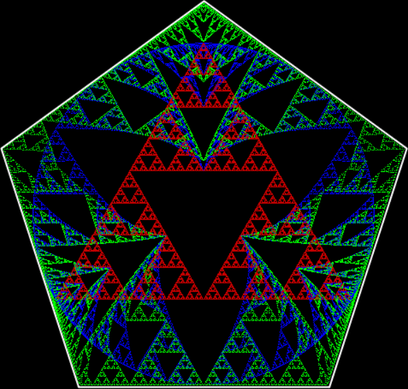
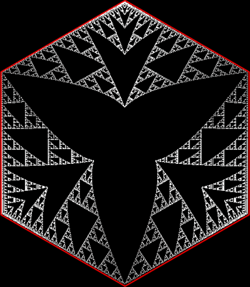
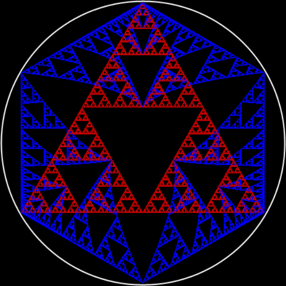
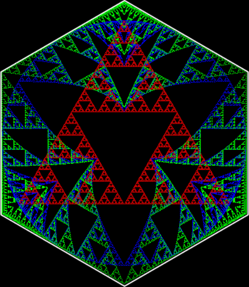
Flowers are modified leaves. That’s a scientific fact. And it must depend on the way the genetic program of a plant allows for change in variables of growth — in the relative dimensions, directions and forms of various collections of cells.

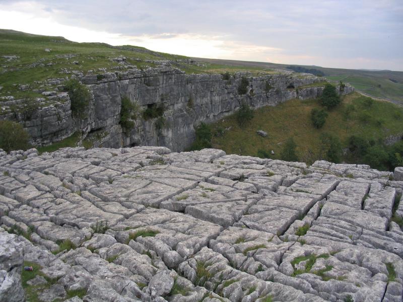
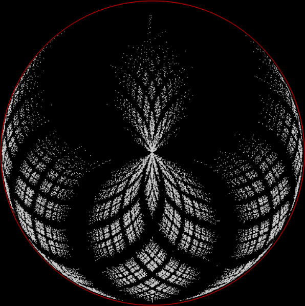
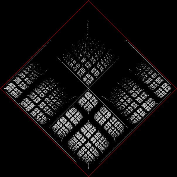
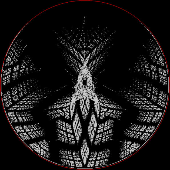
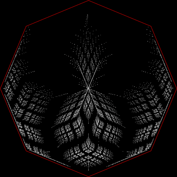
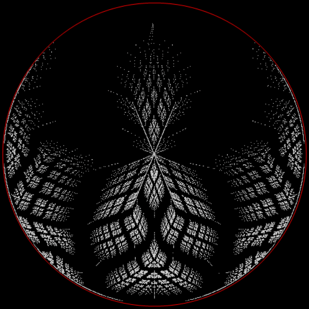
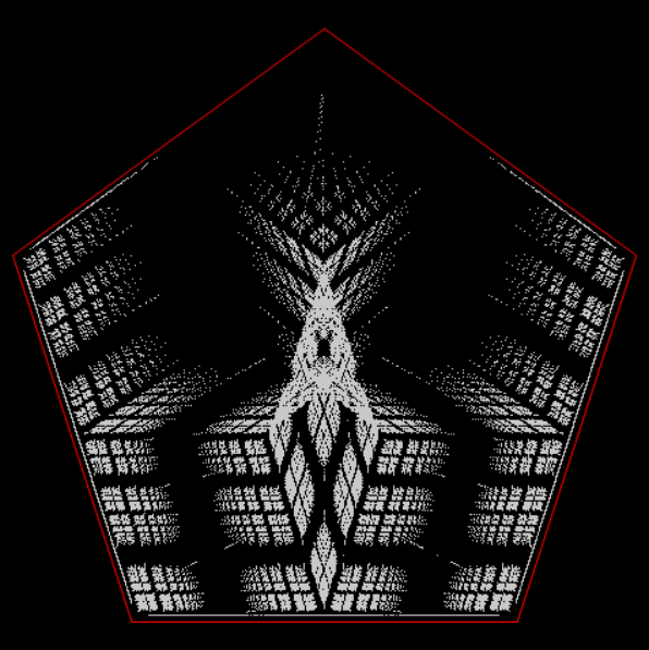
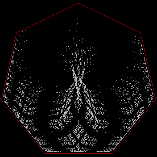
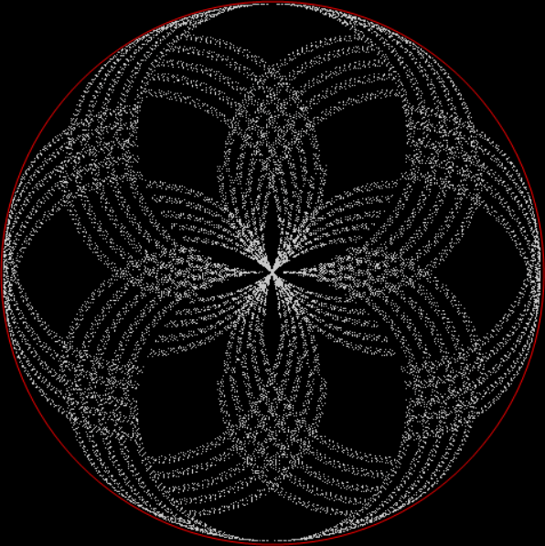
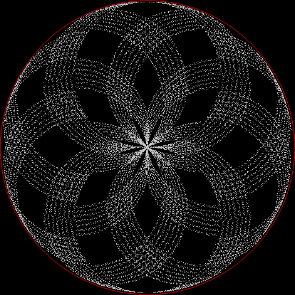
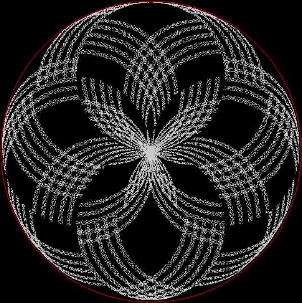
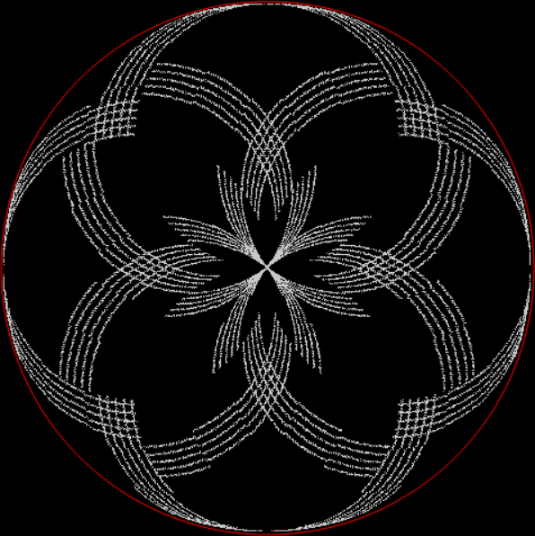
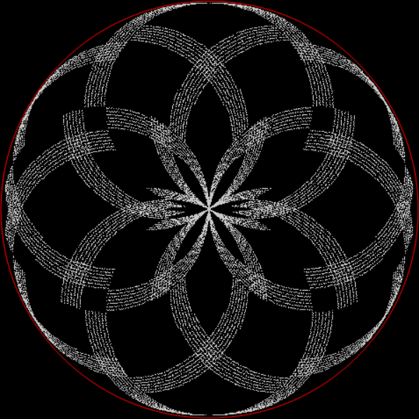
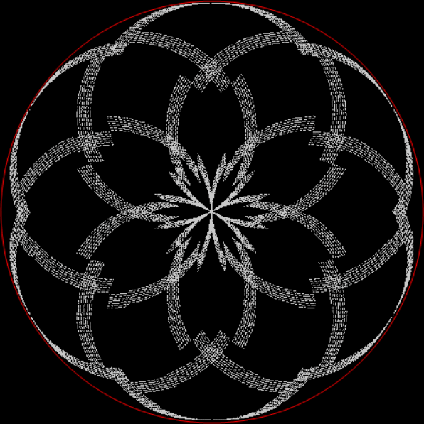
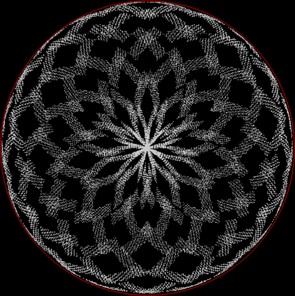
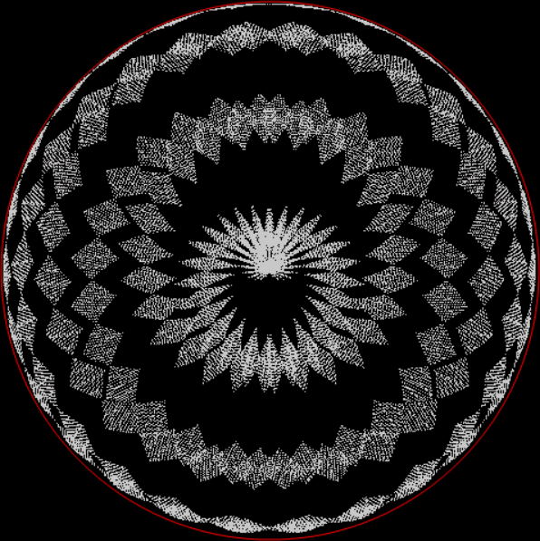
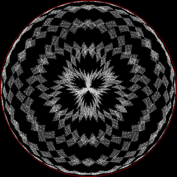
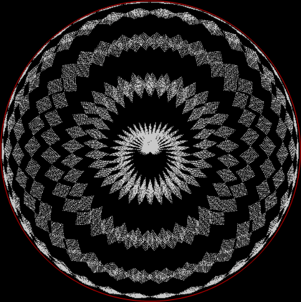
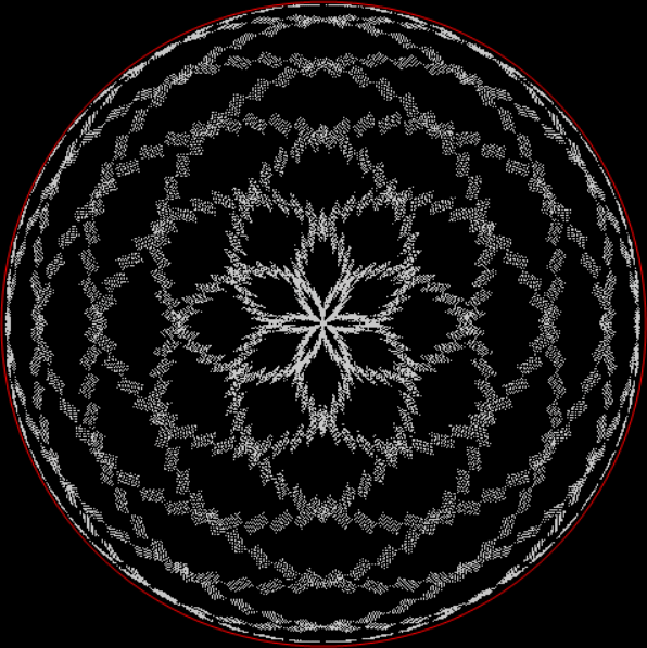
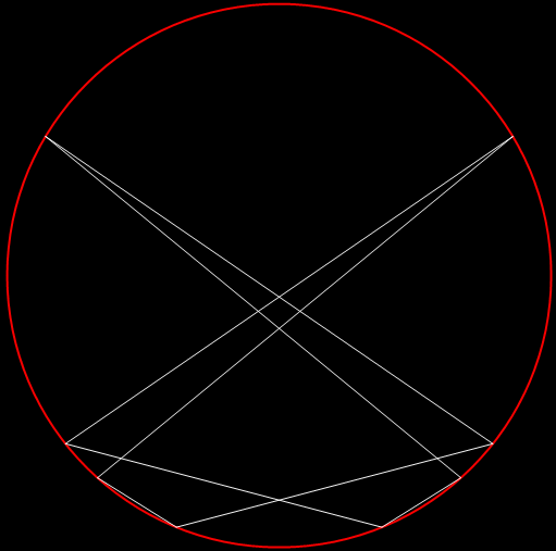
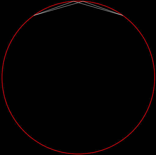
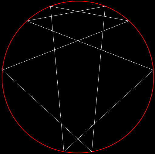
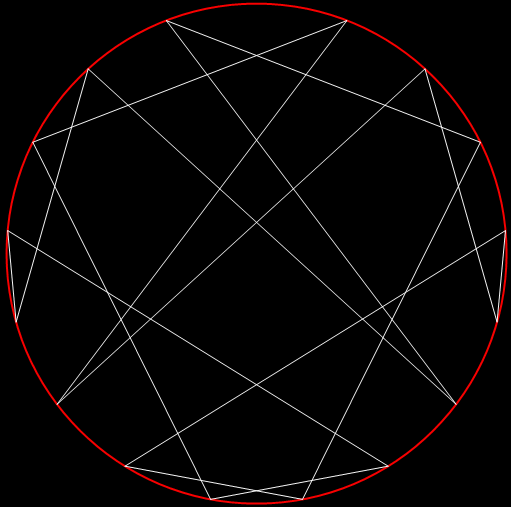
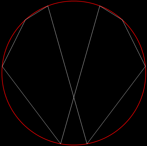
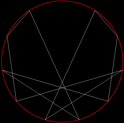
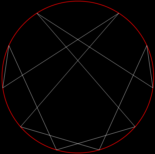
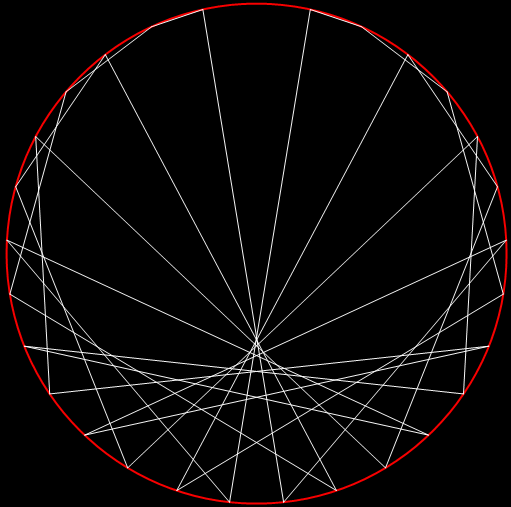
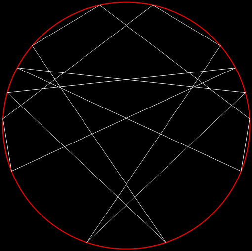
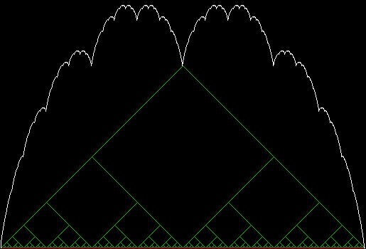
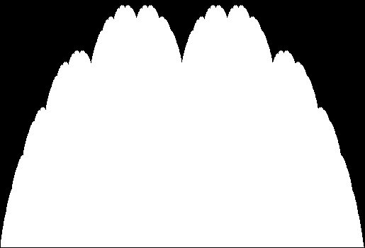
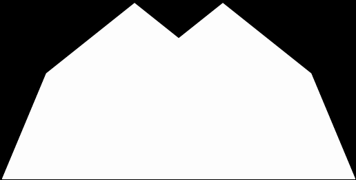
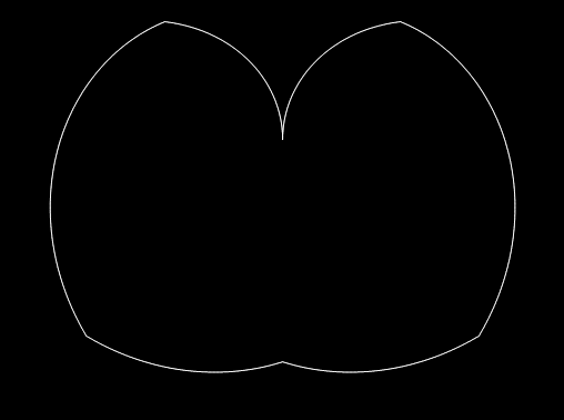
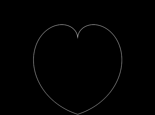
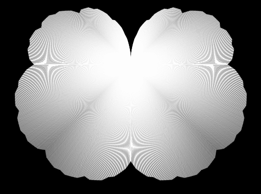
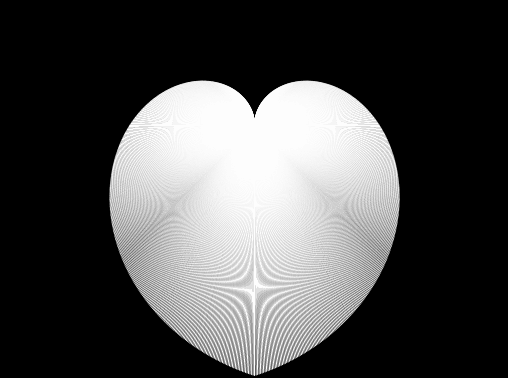
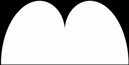
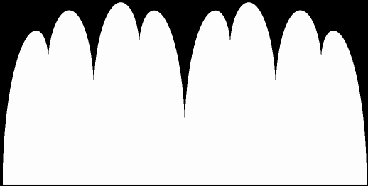
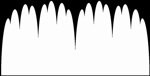
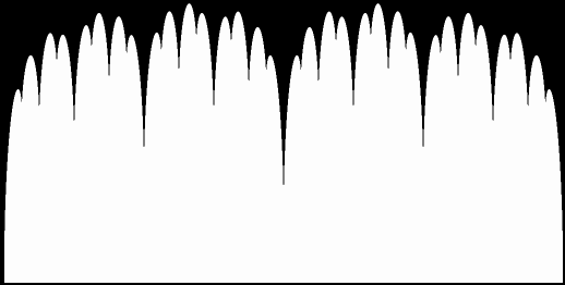
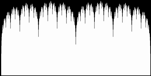
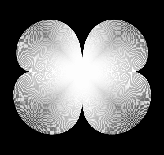
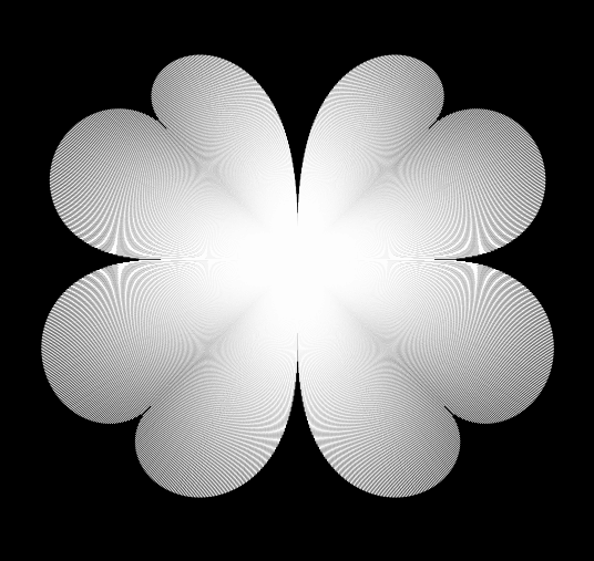
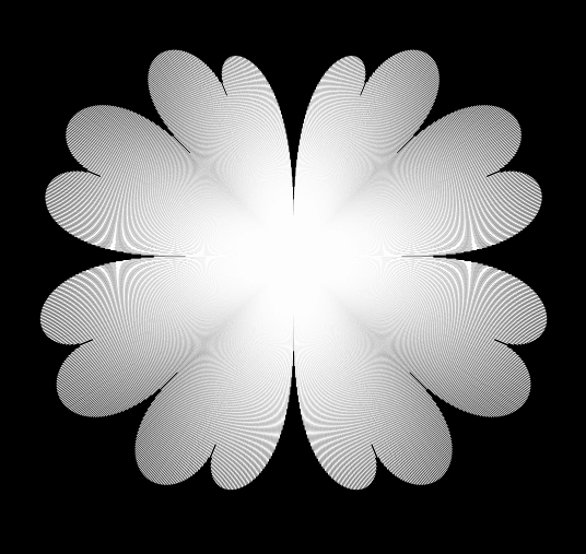
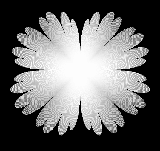
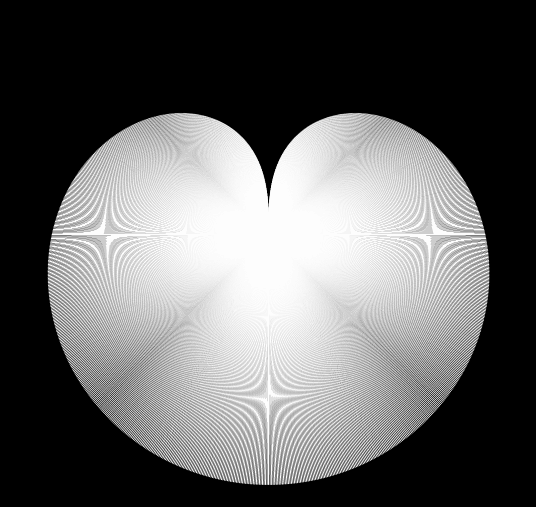
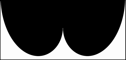
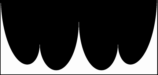
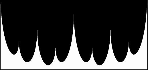
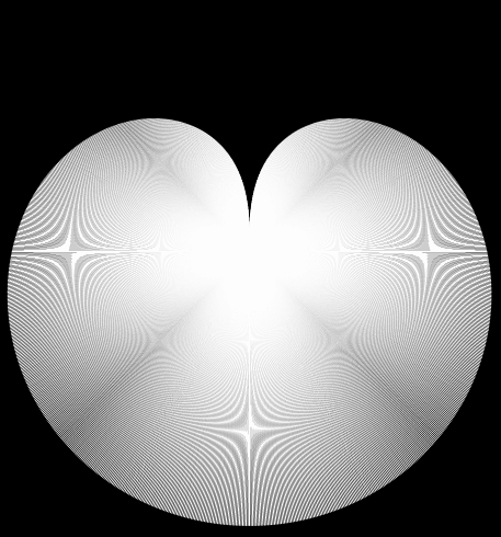
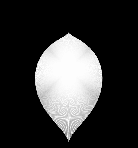
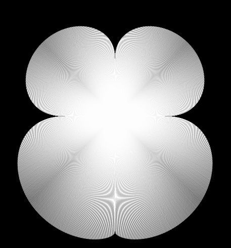
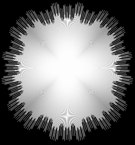
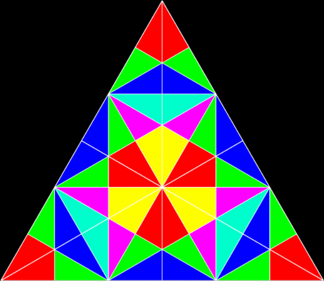
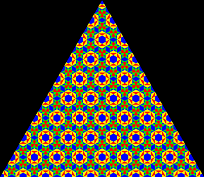
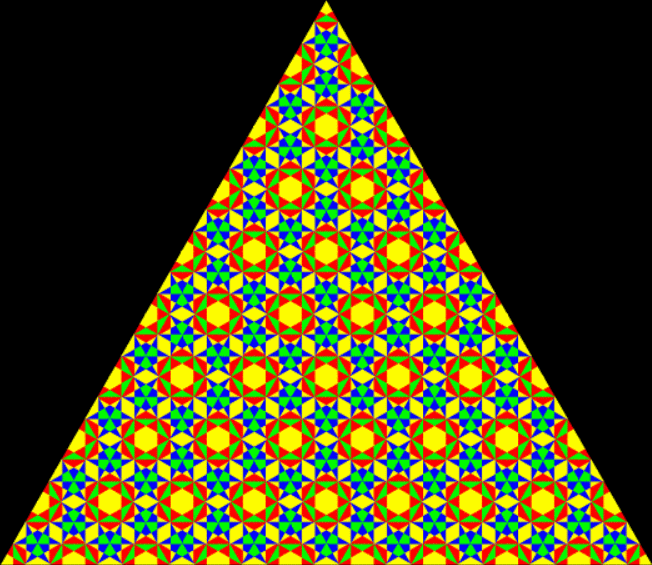
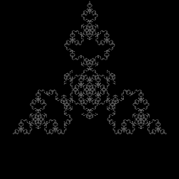
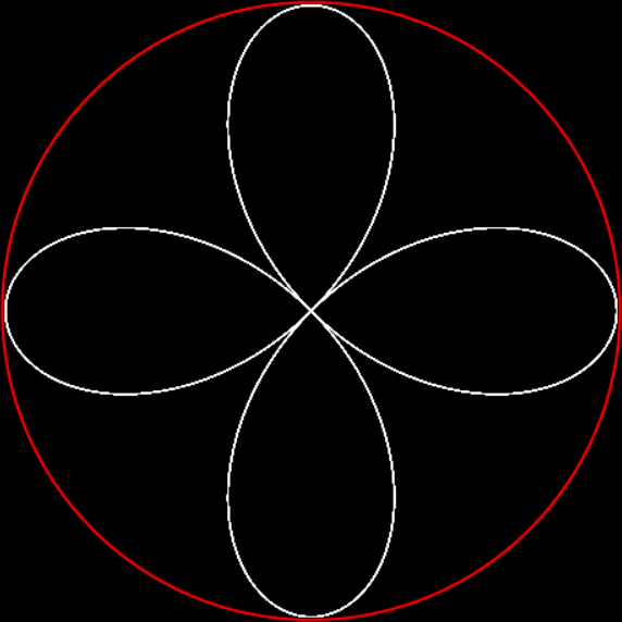
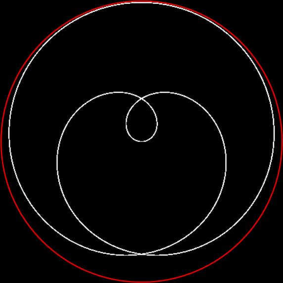
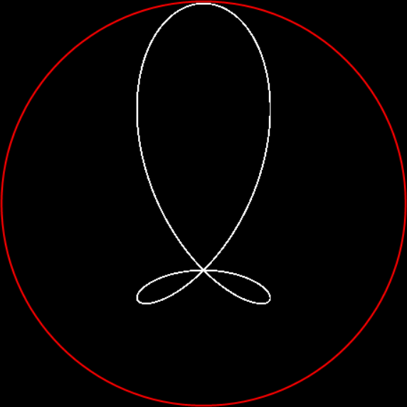
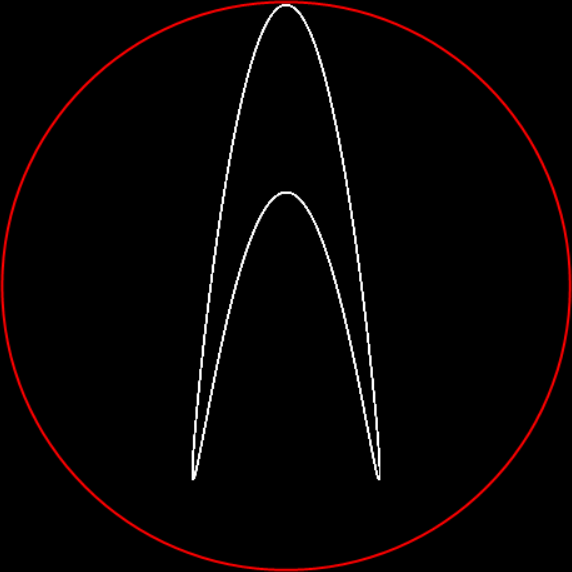
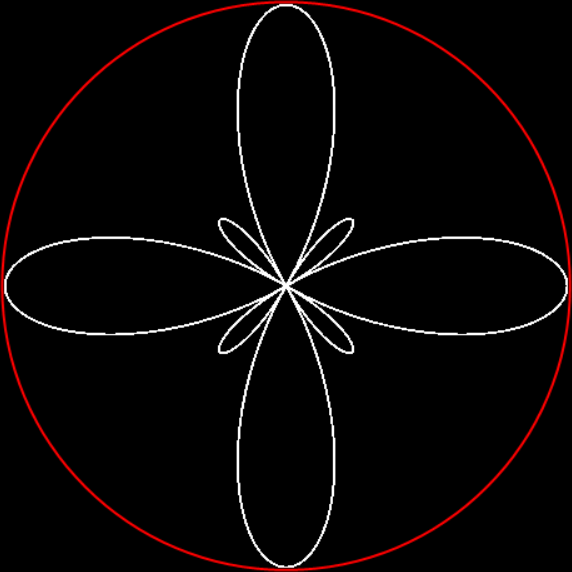
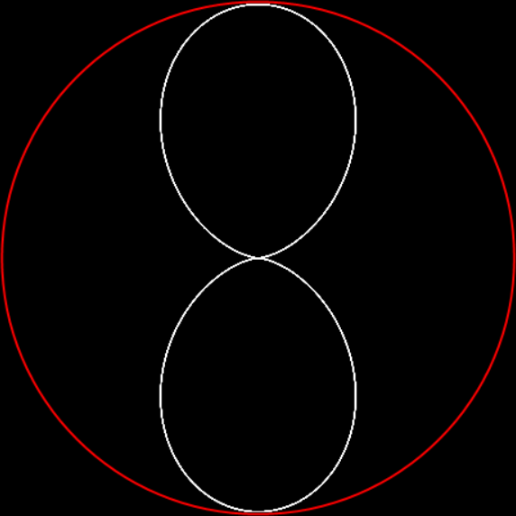
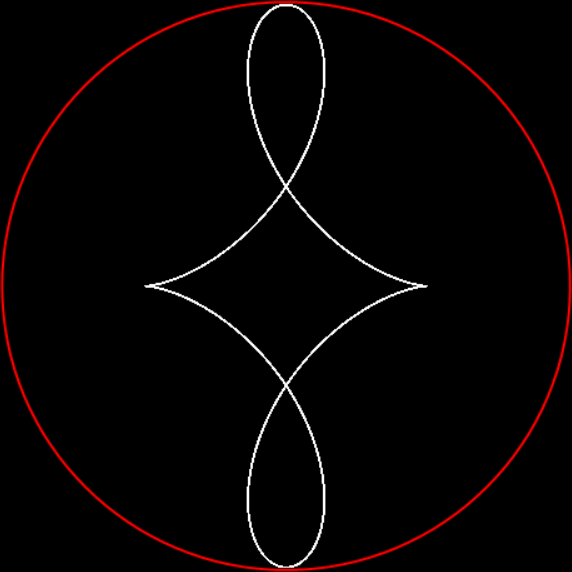
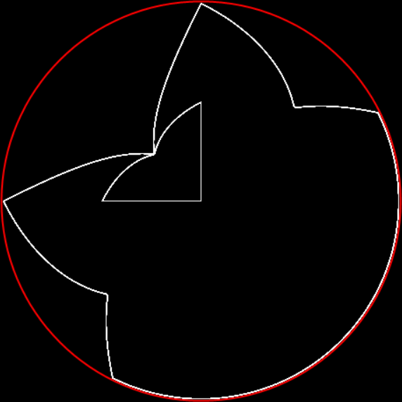
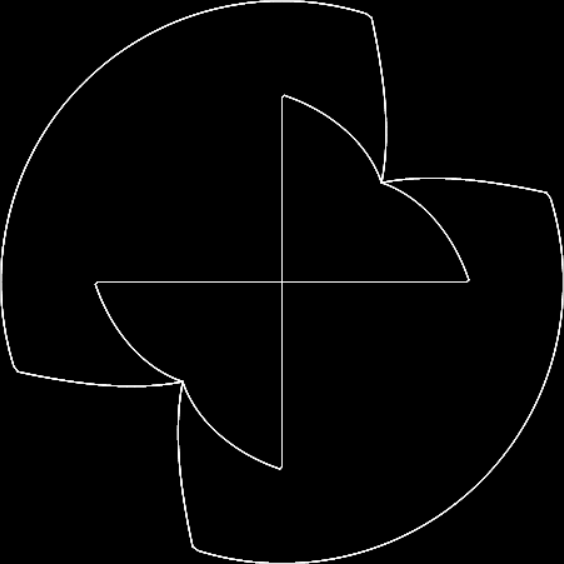
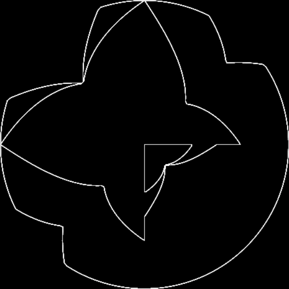
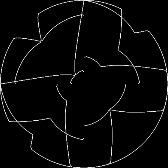
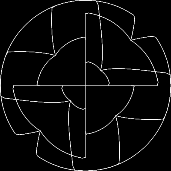
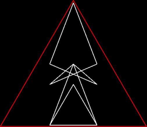
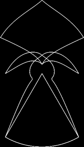
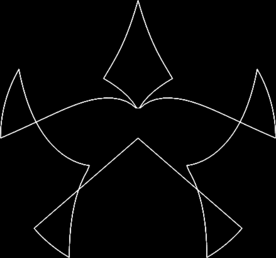
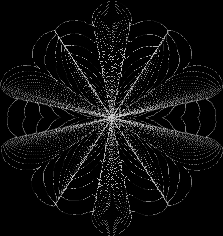
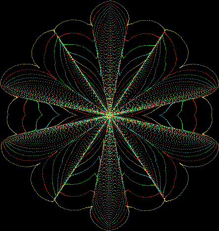
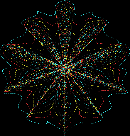
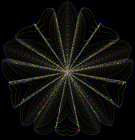
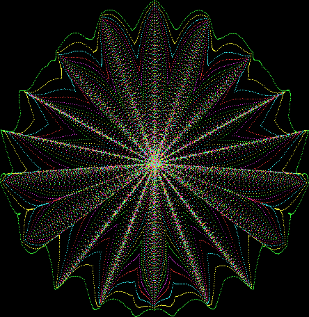
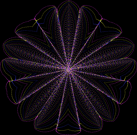
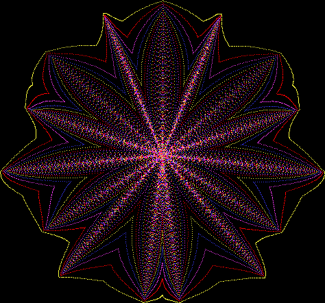
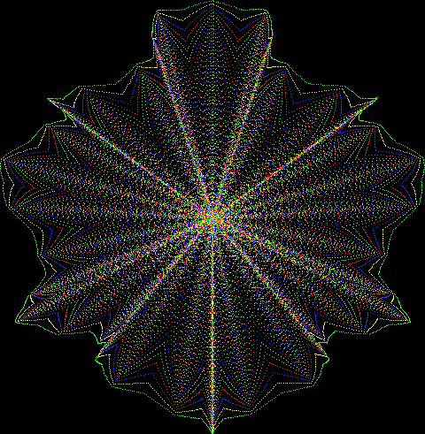
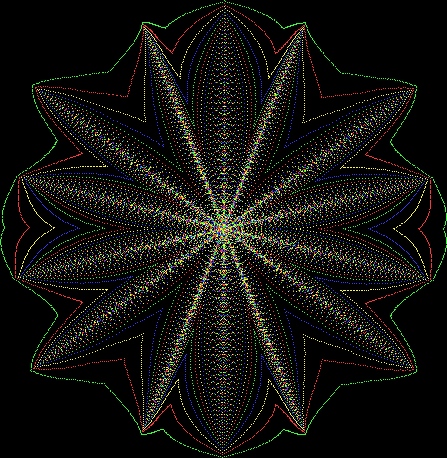
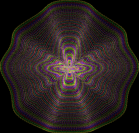
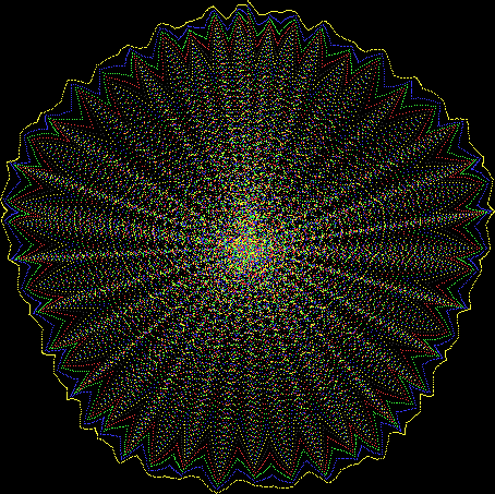
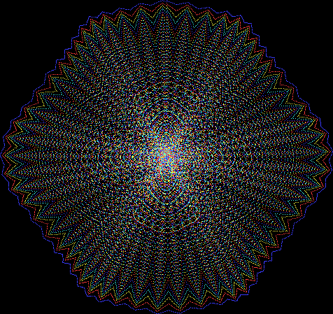
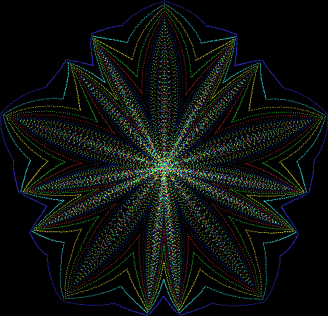
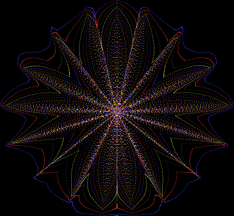
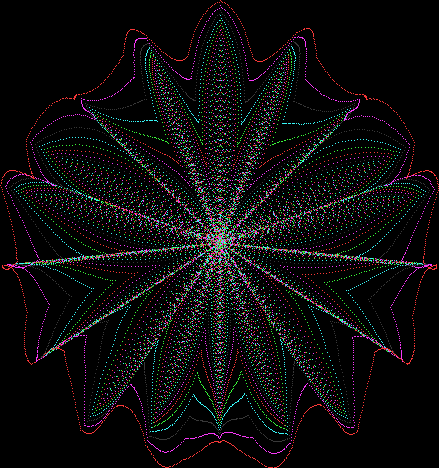
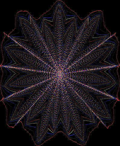
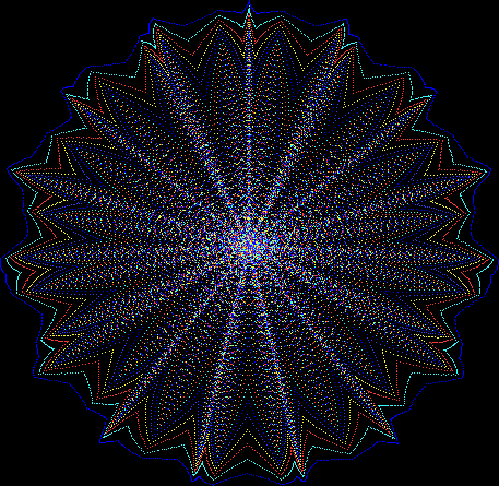
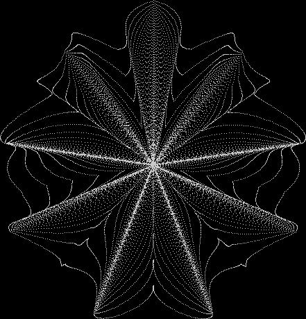
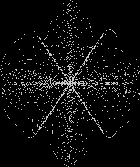
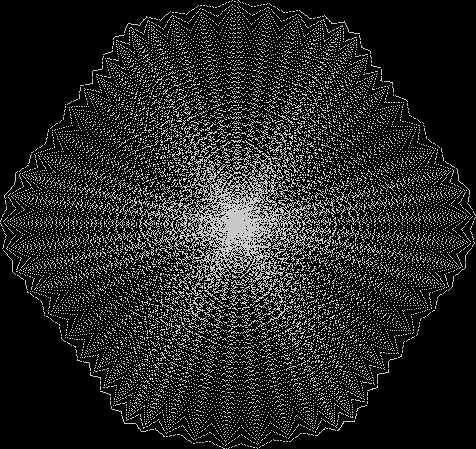
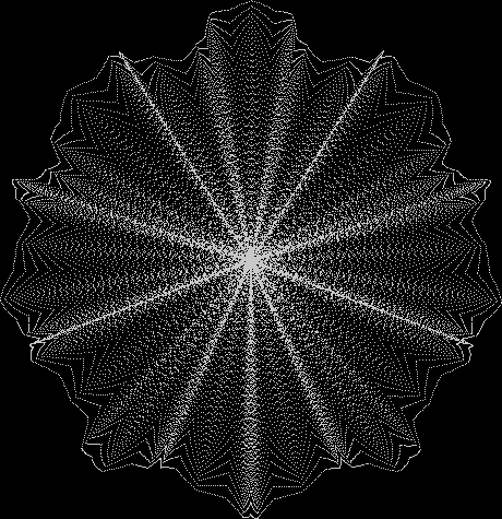
But I wasn’t thinking of flowers or leaves or botany when I wrote a program to trace the path taken by a point moving in various ways between the center and perimeter of a circle. After I’d run the program, I was definitely thinking of flowers and leaves. How could I not be, when they appeared on the screen in front of my eyes? By adjusting variables in the program, I could produce either flowers or leaves or something between the two:

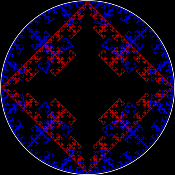
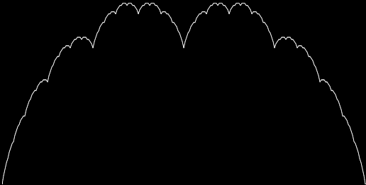
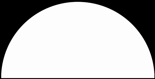
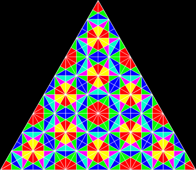
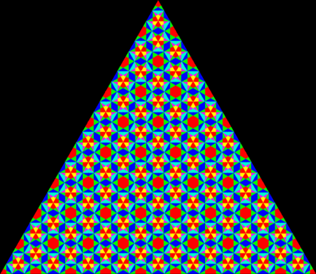
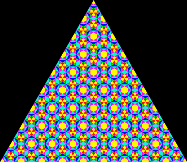
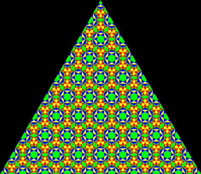
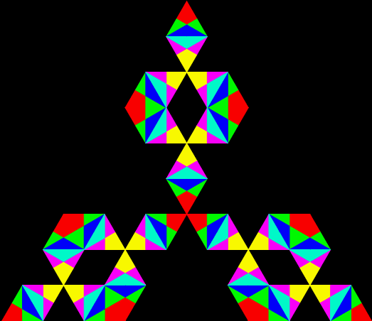
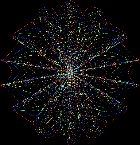
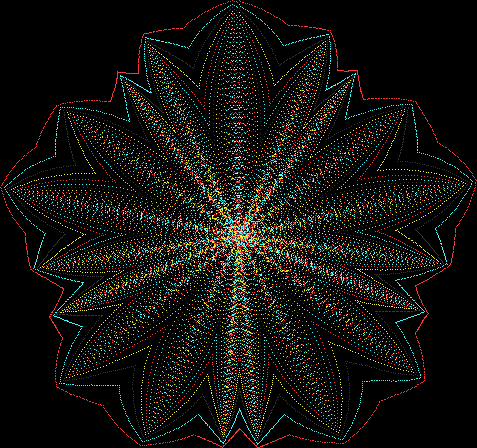
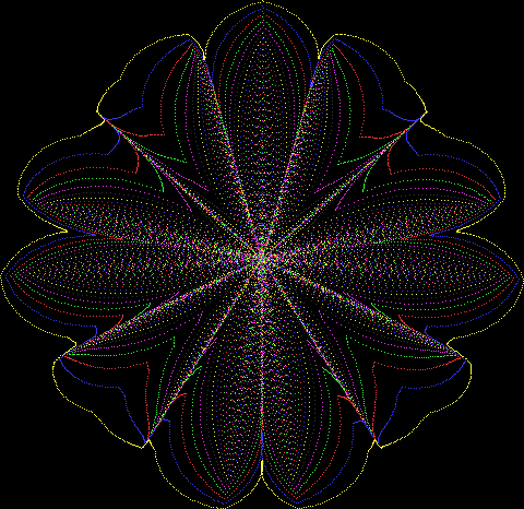
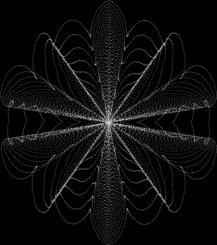
Flower without color
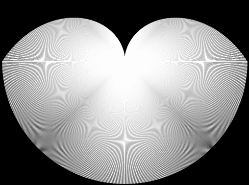
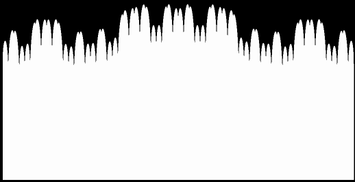
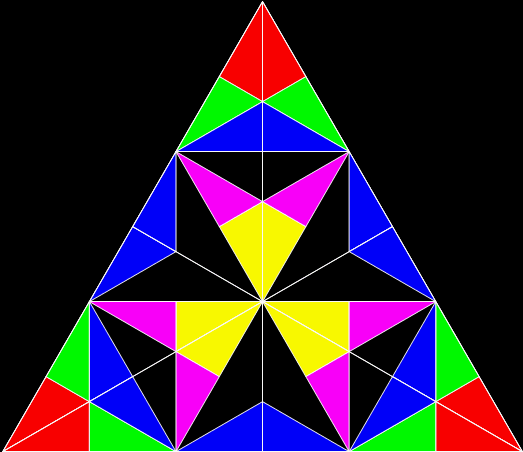
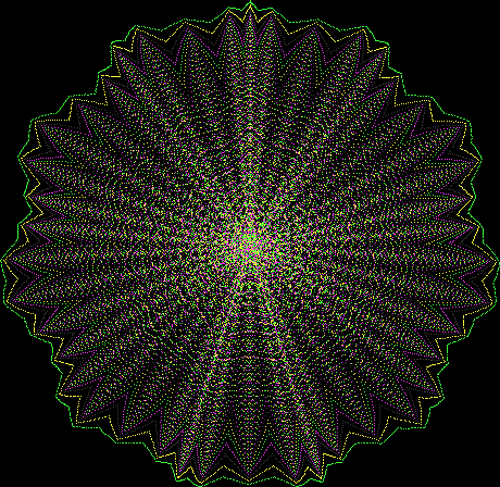
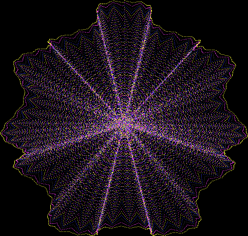
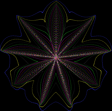

Flower with color


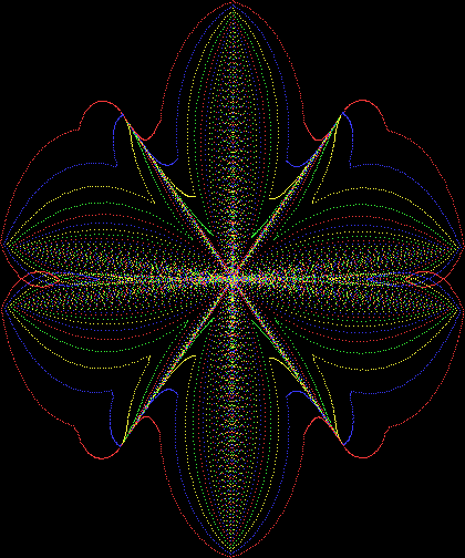
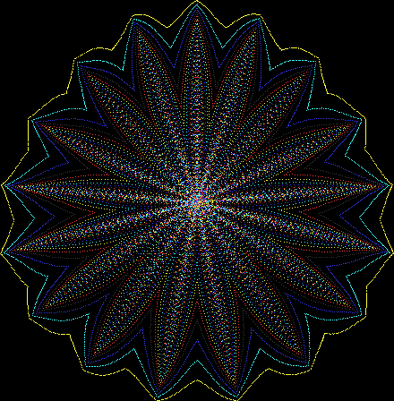
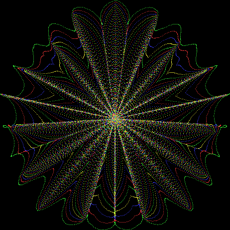
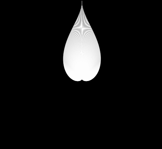
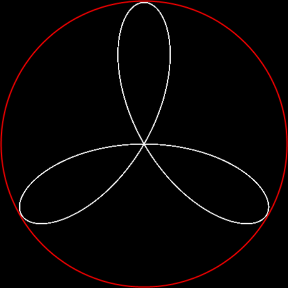
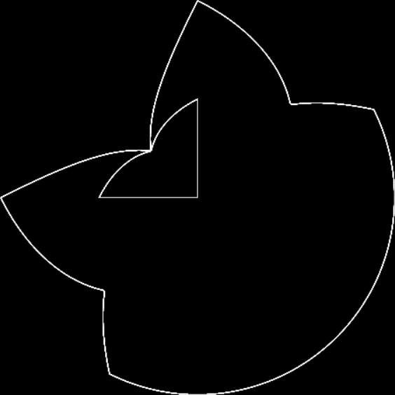
Some of the flower-shapes reminded me of orchids, so I called them mathemorchids. The variables I used governed this procedure:

defprocmathemorchid
rd = 0
jump = jmin
jinc = +1
repeat
xr = xc + int(sin(rd) * rdius + sin(rd * xmult) * xminl)
yr = yc + int(cos(rd) * rdius + cos(rd * ymult) * yminl)
jump = jump + jinc
if(jump = jmin) or (jump >= jmax) then jinc = -jinc
procDrawLine(xr,yr,xc,yc,jump)
rd = rd + rdinc
until rd > maxrd
endproc

Here are explanations of the variables:

rd — short for radian and setting the angle of the point, 0 to maxrd = pi * 2, as it moves between the center and perimeter of the circle
rdinc — the amount by which rd is incremented
xc, yc — the center of the circle
rdius — the radius of the circle
xr, yr — the adjustable radiuses used in trigonometric calculations for the x and y dimensions
xmult, ymult — used to multiply rd for further trig-calcs using…
xminl, yminl — the lengths by which xr and yr are adjusted
jmin, jmax — these are the lower and upper bounds for a rising and falling variable called jump, which determines how far the point moves before it’s marked on the screen

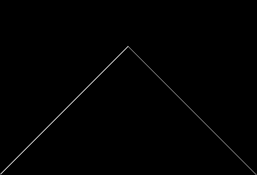
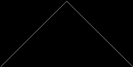
If you look at the use of the sine and cosine functions, you’ll see that the point can swing back on its path or swing ahead of itself, as it were. That’s how the path of the point can simulate three-dimensionality as it lays down thicker or thinner patches of pixels.

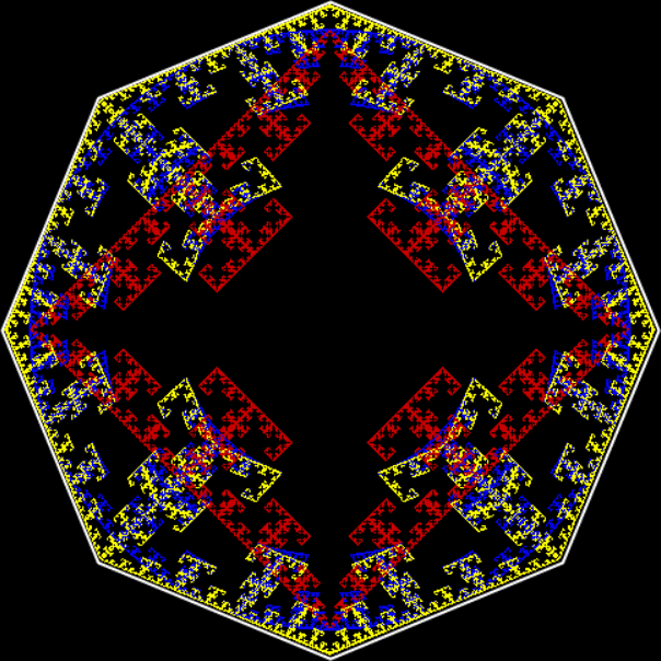
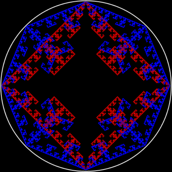
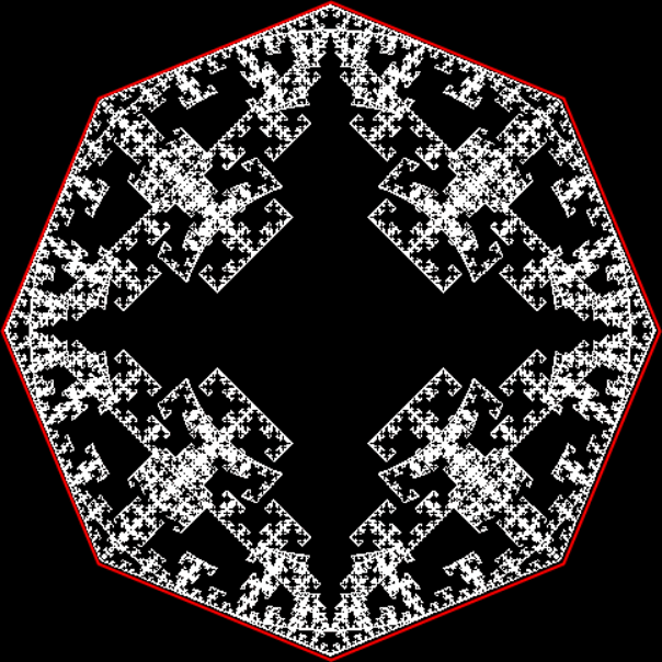
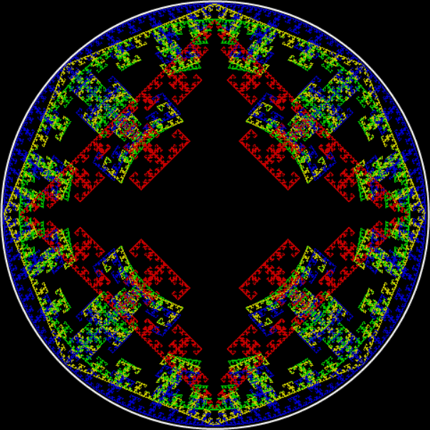
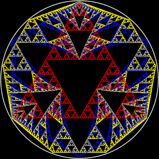
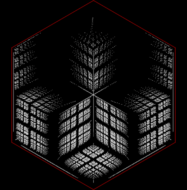
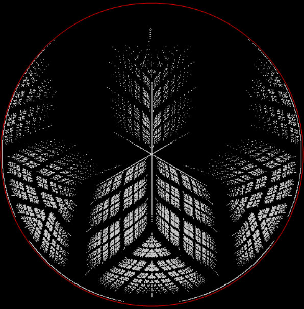
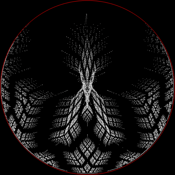
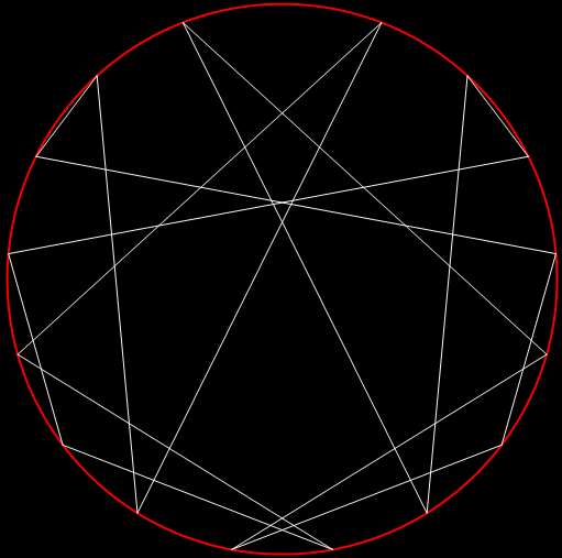
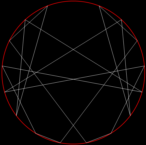
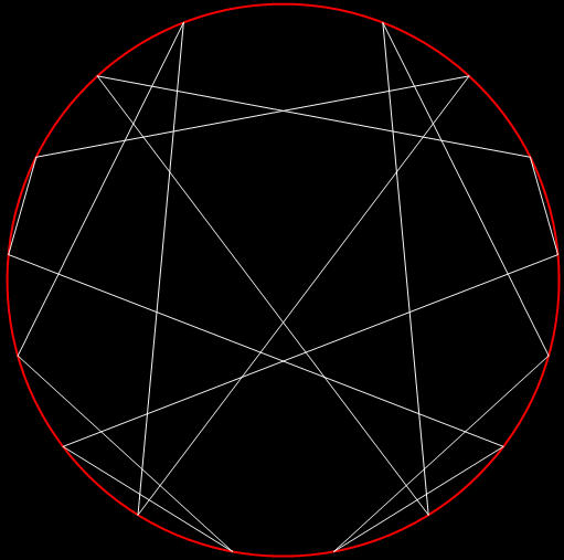
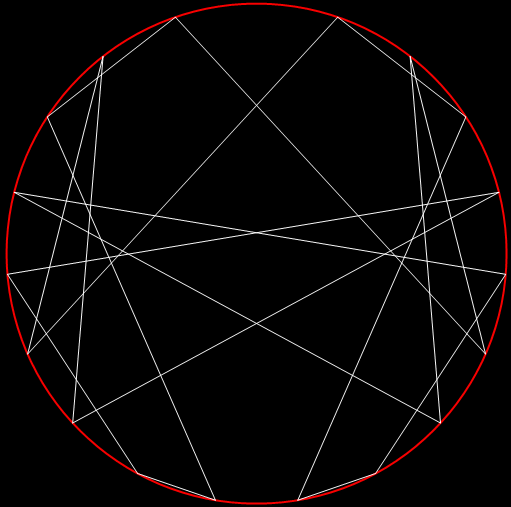
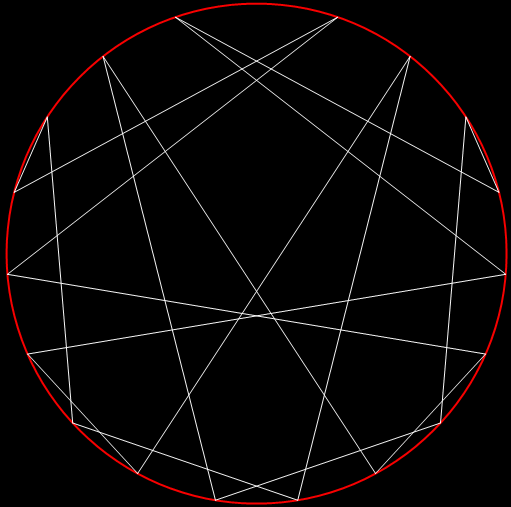
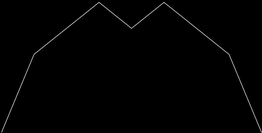
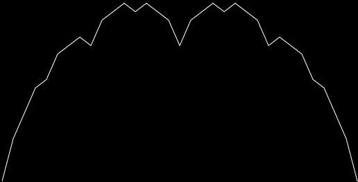
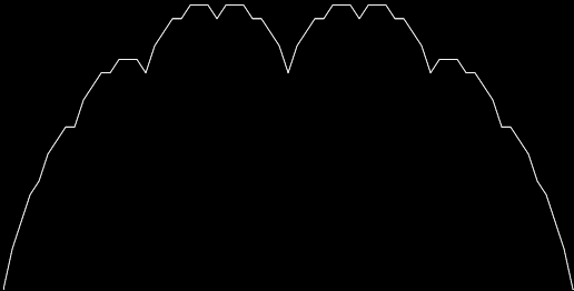
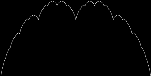
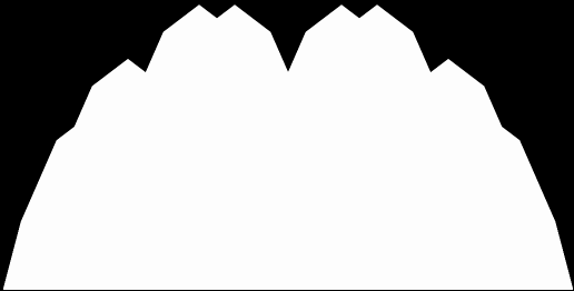
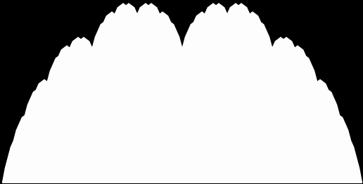
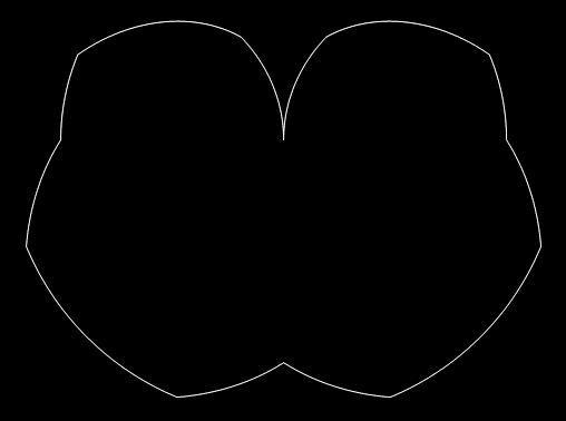
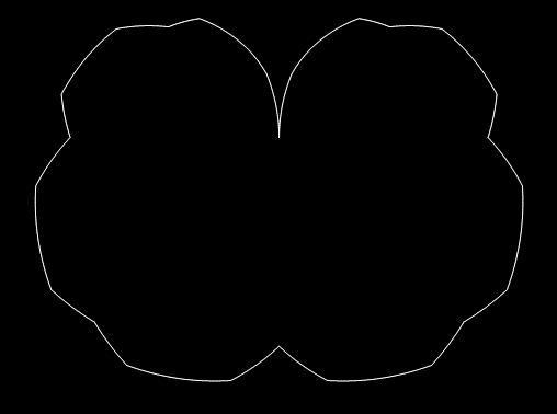
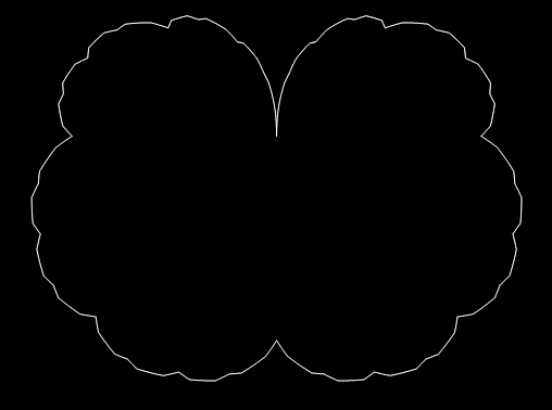
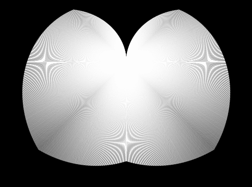
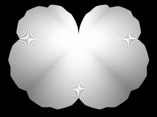
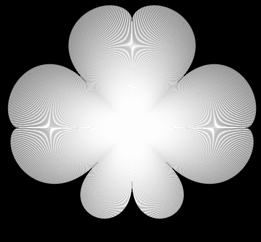
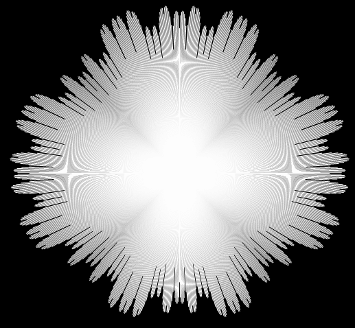
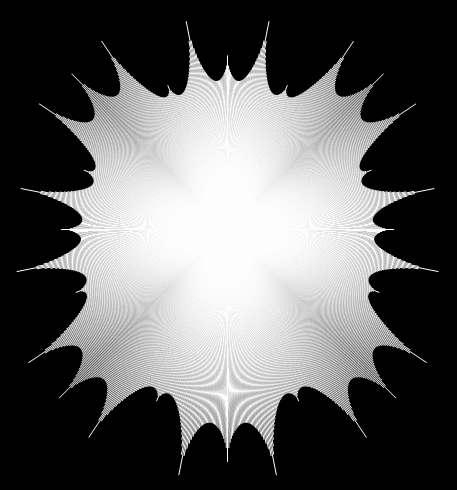
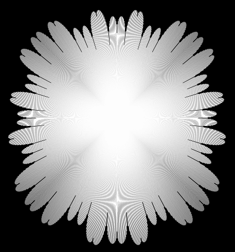
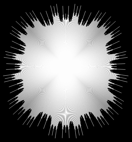
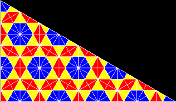
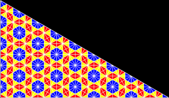
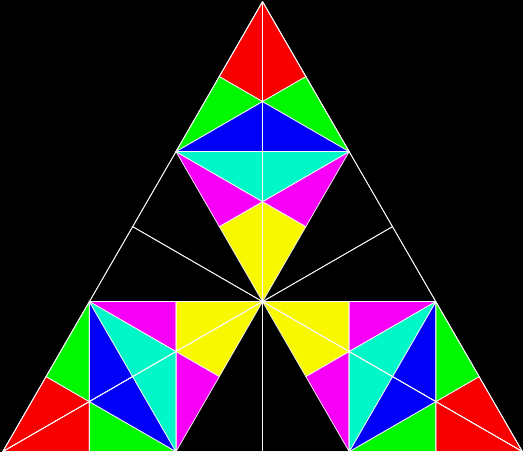
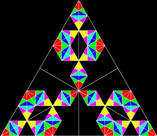
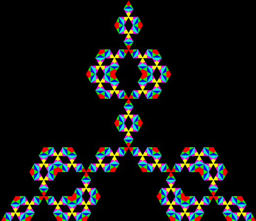
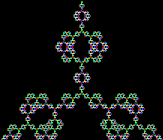
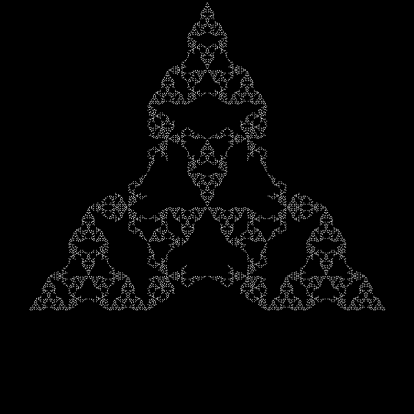
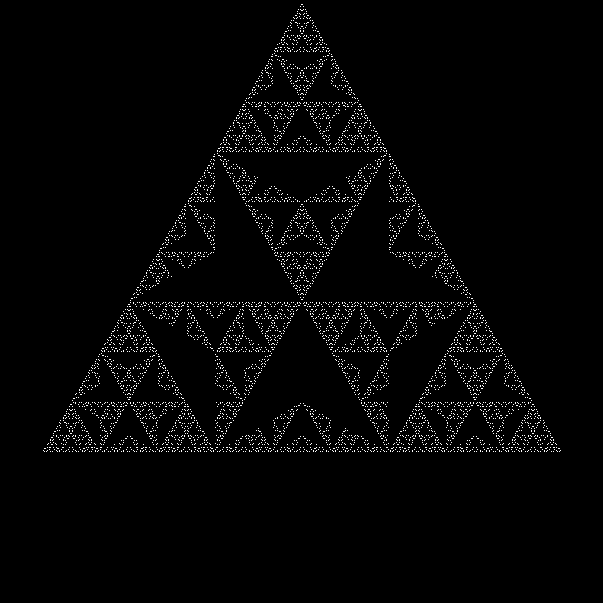
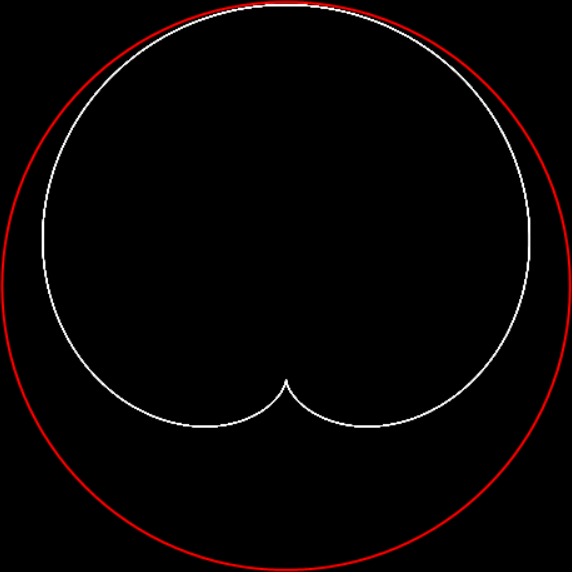
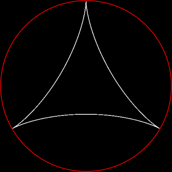
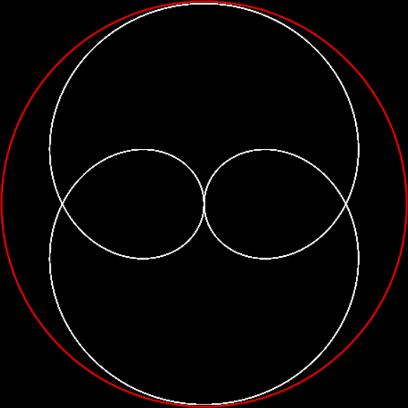
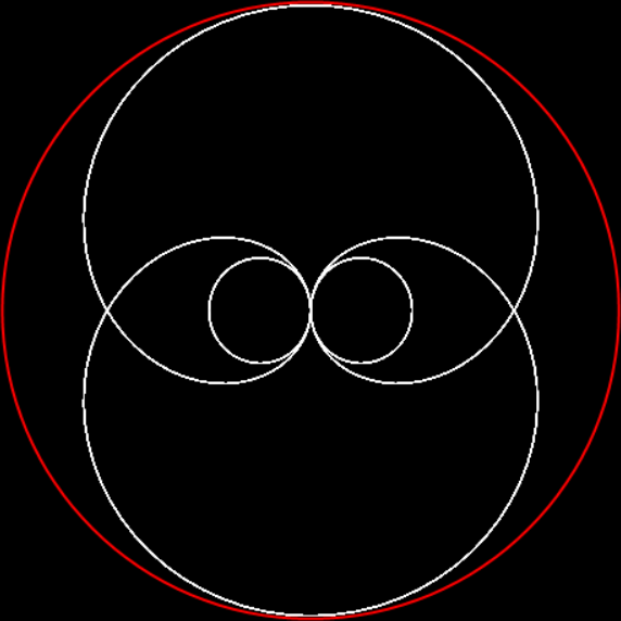
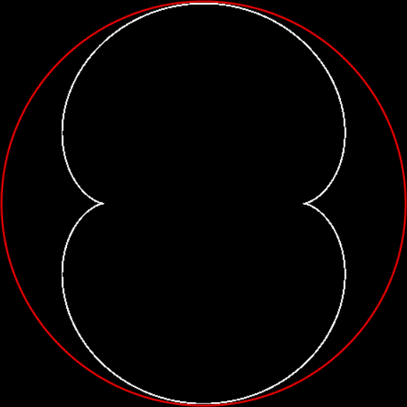
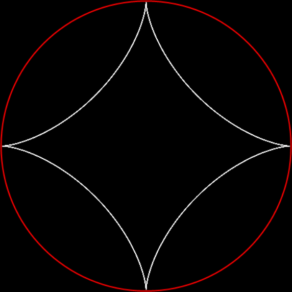
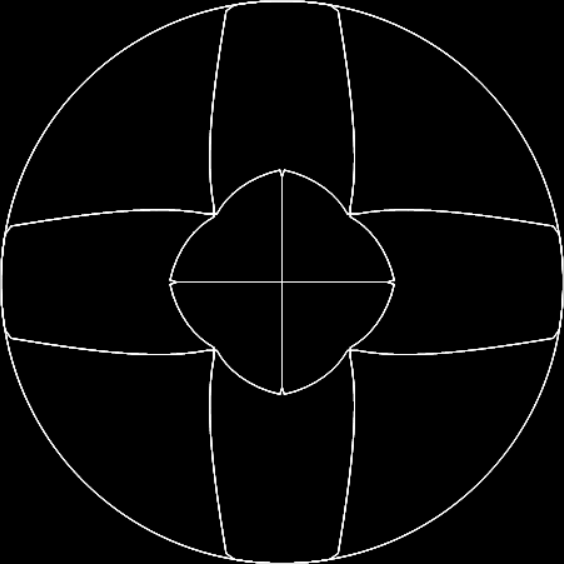
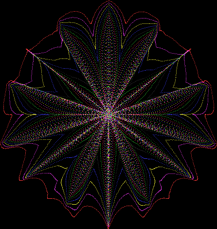
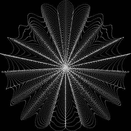
Here are the mathemorchids, leaves, scallops and other shapes created by adjusting the variables described above (with more of the generating program as an appendix):

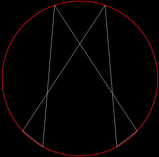
Mathemorchid for jmin = 6, jmax = 69, xmult = 7, ymult = 7, xminl = 40, yminl = 88 (see file-name)


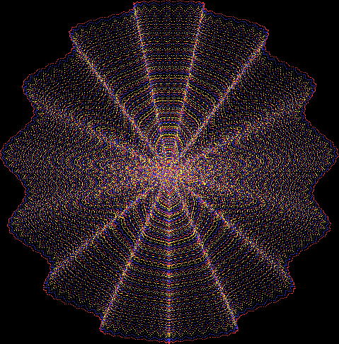
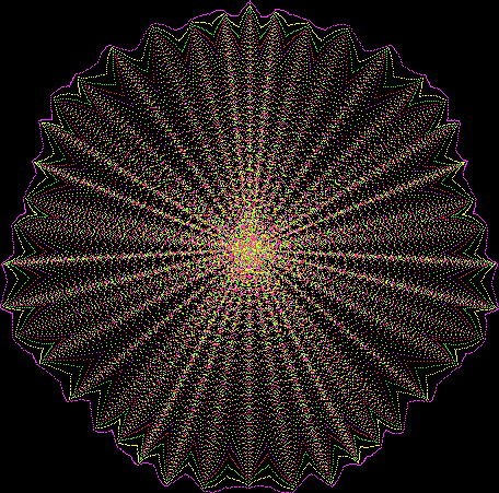
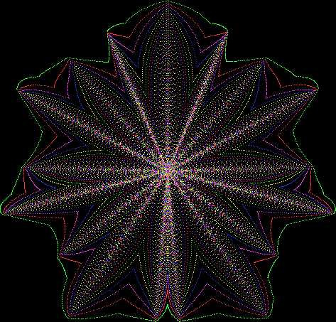
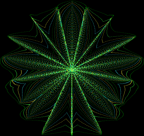
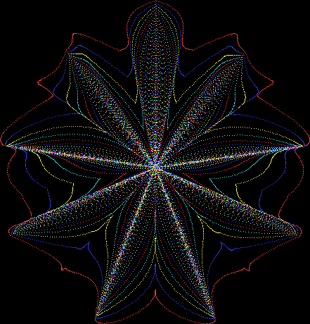
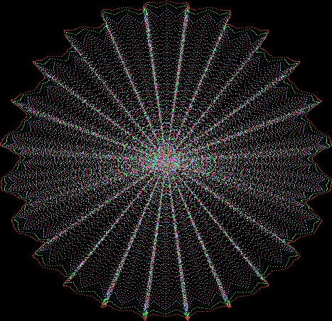
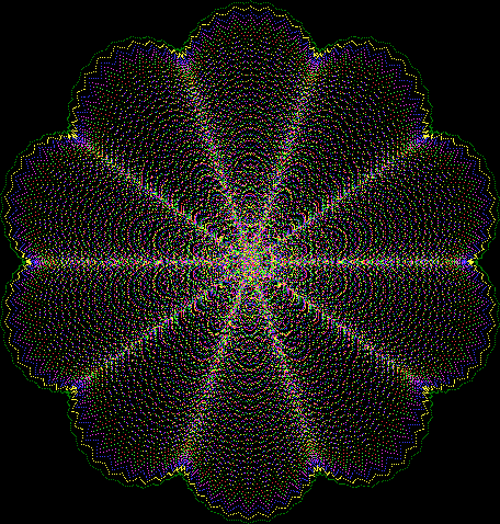
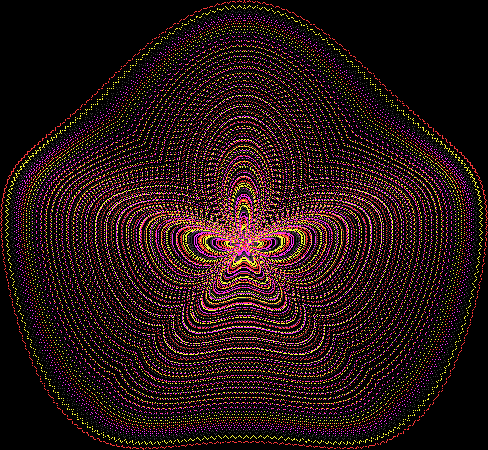
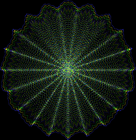
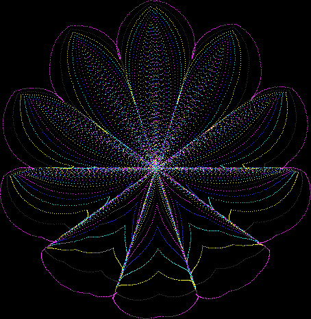
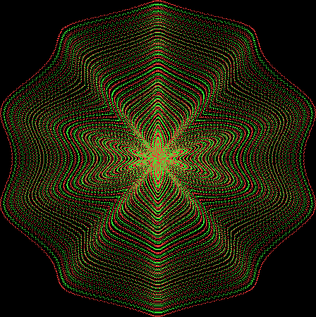
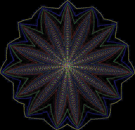
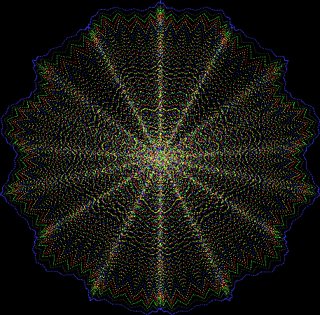
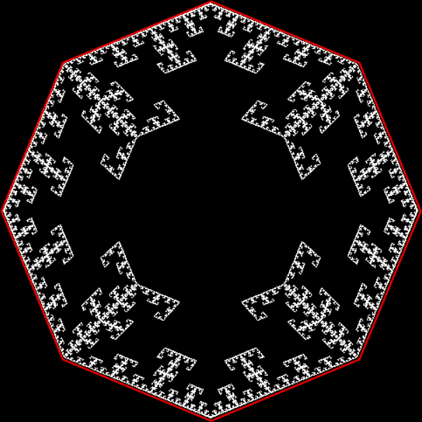
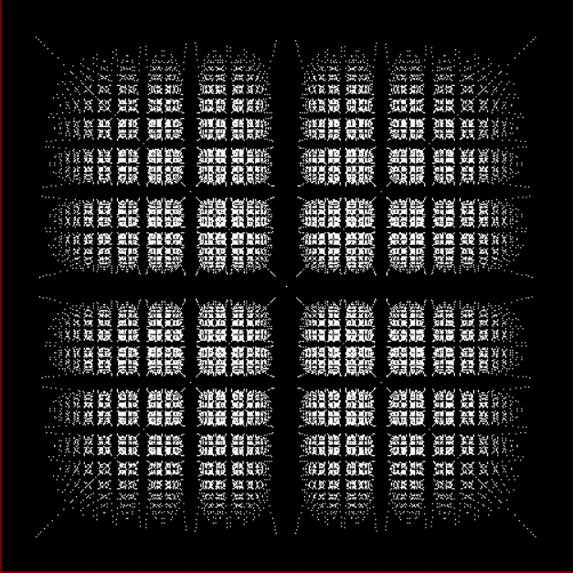
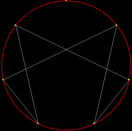
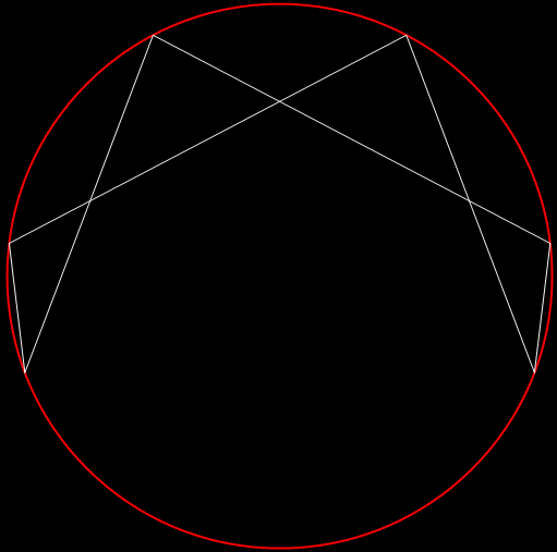
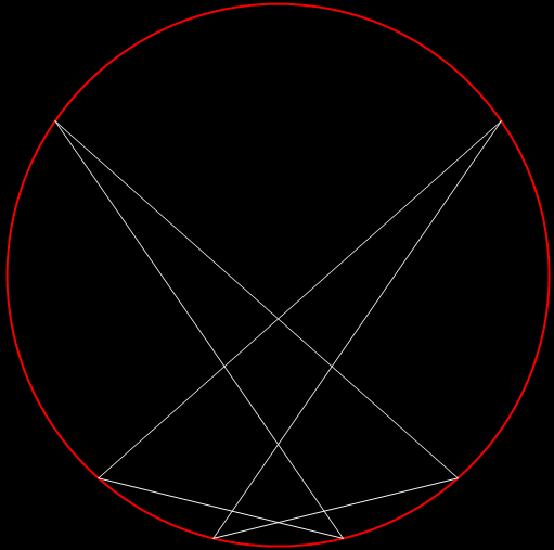
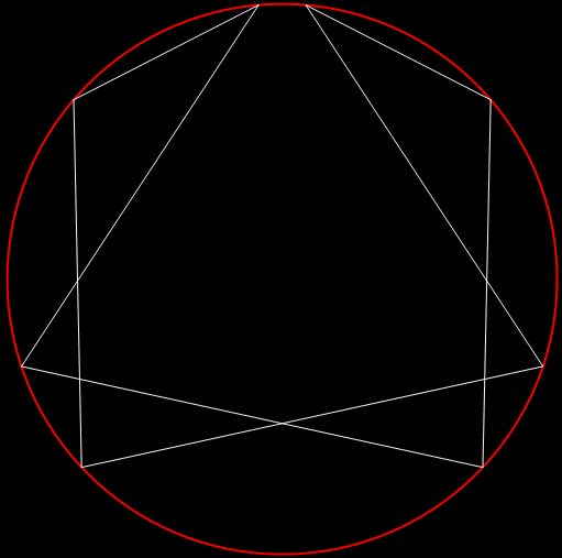
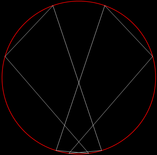
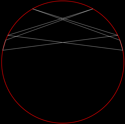
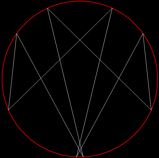
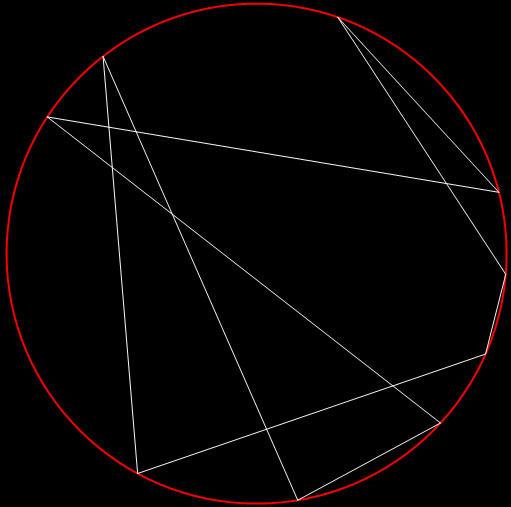
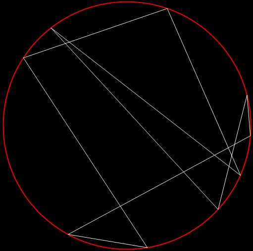
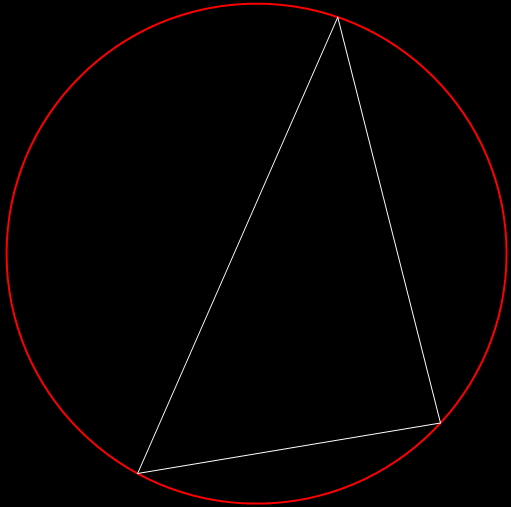
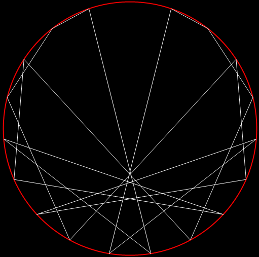
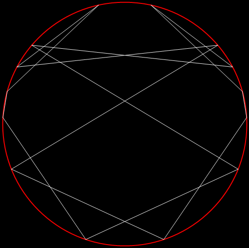
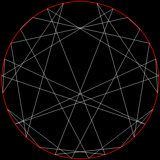
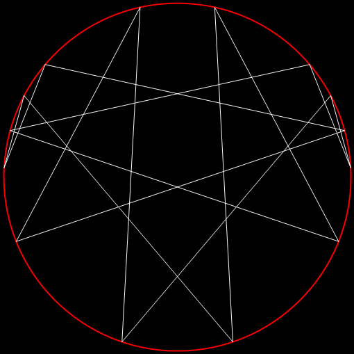
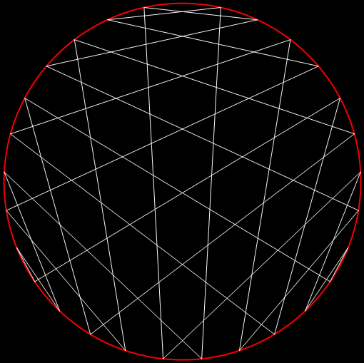
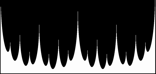
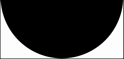
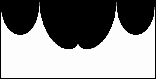
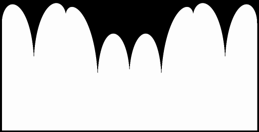
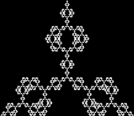
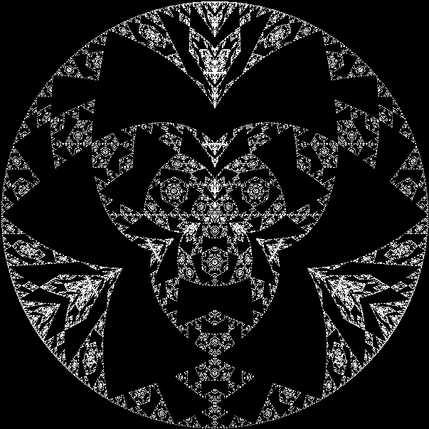
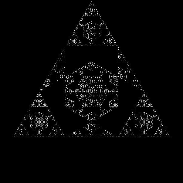
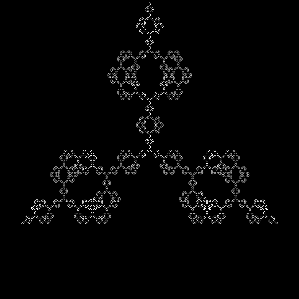
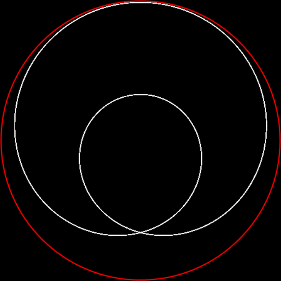
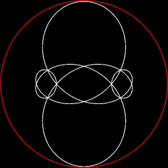
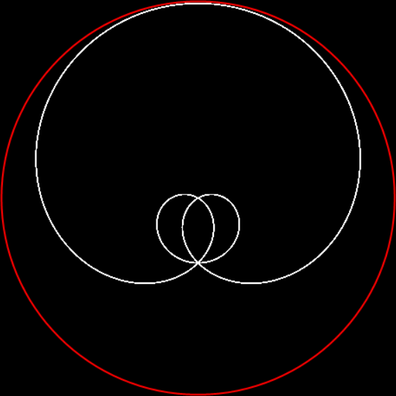
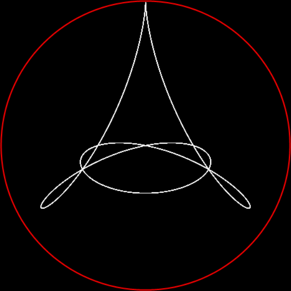
And here are a few more examples of the mathemorchids and other shapes look like without color:


Code for creating the Mathemorchids

defprocmathemorchid
rd = 0
rd = 0
jump = jmin
jinc = +1
repeat
xr = xc + int(sin(rd) * rdius + sin(rd * xmult) * xminl)
yr = yc + int(cos(rd) * rdius + cos(rd * ymult) * yminl)
jump = jump + jinc
if(jump = jmin) or (jump >= jmax) then jinc = -jinc
procDrawLine(xr,yr,xc,yc,jump)
rd = rd + rdinc
k=inkey(0)
until rd > maxrd or k > -1
endproc

defprocDrawLine(x1,y1,x2,y2,puttest)
xdiff = x1 – x2
ydiff = y1 – y2
if abs(xdiff) > abs(ydiff) then
yinc = -ydiff / abs(xdiff)
if xdiff < 0 then xinc = +1 else xinc = -1
else
xinc = -xdiff / abs(ydiff)
if ydiff colrmx then col = 1
put = 0
endif
if int(x) x2 then x = x + xinc
if int(y) y2 then y = y + yinc
iffunc=2then
ifx<x_lo x_lo=x
ifyx_hi x_hi=x
ify>y_hi y_hi=y
endif
until fnreached
endproc

deffnreached
if xinc > 0 then
xreached = int(x) >= x2
else
xreached = int(x) 0 then
yreached = int(y) >= y2
else
yreached = int(y) <= y2
endif
= xreached and yreached
end

Squaring the Triangle

It’s an interesting little exercise in elementary trigonometry to turn the Sierpiński triangle…

A Sierpiński triangle


…into its circular equivalent:

A Sierpiński trisc


You could call that a trisc, because it’s a triangle turned into a disc. And here’s triangle-and-trisc in one image:

Sierpiński triangle + Sierpiński trisc


But what’s the square equivalent of a Sierpiński triangle? This is:

Square from Sierpiński triangle


You can do that directly, as it were:

Sierpiński triangle → square


Or you can convert the triangle into a disc, then the disc into a square, like this:

Sierpiński triangle → trisc → square


Now try converting the triangle into a pentagon:

Pentagon from Sierpiński triangle


Sierpiński triangle → pentagon


Sierpiński triangle → trisc → pentagon


And a hexagon:

Hexagon from Sierpiński triangle


Sierpiński triangle → hexagon


Sierpiński triangle → trisc → hexagon


But you can also convert the Sierpiński trisc back into a Sierpiński triangle, then into a Sierpiński trisc again:

Sierpiński triangle → trisc → triangle → trisc


Sierpiński triangle → trisc → triangle → trisc (animated at Ezgif)


Sierpiński triangle → trisc → triangle → trisc (b&w)


Sierpiński triangle → trisc → triangle → trisc (b&w) (animated at Ezgif)


After triangles come squares. Here’s a shape called a T-square fractal:

T-square fractal


And here’s the circular equivalent of a T-square fractal:

T-square fractal → T-squisc


T-square fractal + T-squisc


If a disc from a triangle is a trisc, then a disc from a square is a squisc (it would be pentisc, hexisc, heptisc for pentagonal, hexagonal and heptagonal fractals). Here’s the octagonal equivalent of a T-square fractal:

Octagon from T-square fractal


As with the Sierpiński trisc, you can use the T-squisc to create the T-octagon:

T-square fractal → T-squisc → T-octagon (color)


Or you can convert the T-square directly into the T-octagon:

T-square fractal to T-octagon fractal

But using the squisc makes for interesting multiple images:


T-square fractal → T-squisc → T-octagon (b&w)


T-square fractal → T-squisc → T-octagon → T-squisc


T-square fractal → T-squisc → T-octagon → T-squisc (animated at Ezgif)


The conversions from polygon to polygon look best when the number of sides in the higher polygon are a multiple of the number of sides in the lower, like this:

Sierpiński triangle → Sierpiński hexagon → Sierpiński nonagon


Lime Time

What do you get if you list every successive pair of entries in this sequence?

1, 2, 1, 3, 2, 3, 1, 4, 3, 4, 1, 5, 2, 5, 3, 5, 4, 5, 1, 6, 5, 6, 1, 7, 2, 7, 3, 7, 4, 7, 5, 7, 6, 7, 1, 8, 3, 8, 5, 8, 7, 8, 1, 9, 2, 9, 4, 9, 5, 9, 7, 9, 8, 9, 1, 10, 3, 10, 7, 10, 9, 10, 1, 11, 2, 11, 3, 11, 4, 11, 5, 11, 6, 11, 7, 11, 8, 11, 9, 11, 10, 11, 1, 12, 5, 12, 7, 12, 11, 12, 1, 13, … — A038568 at the Online Encyclopedia of Integer Sequence

You get the rational fractions ordered by denominator in their simplest form: 1/2, 1/3, 2/3, 1/4, 3/4, 1/5, 2/5, 3/5… There are no pairs like 2/4 and 5/35, because those can be simplified: 2/4 → 1/2; 15/35 → 3/7. You can get the same set of rational fractions by listing every successive pair in this sequence, the Stern-Brocot sequence:

1, 2, 1, 3, 2, 3, 1, 4, 3, 5, 2, 5, 3, 4, 1, 5, 4, 7, 3, 8, 5, 7, 2, 7, 5, 8, 3, 7, 4, 5, 1, 6, 5, 9, 4, 11, 7, 10, 3, 11, 8, 13, 5, 12, 7, 9, 2, 9, 7, 12, 5, 13, 8, 11, 3, 10, 7, 11, 4, 9, 5, 6, 1, 7, 6, 11, 5, 14, 9, 13, 4, 15, 11, 18, 7, 17, 10, 13, 3, 14, 11, 19, 8, 21, 13, 18, 5, 17, 12, 19, … — A002487 at the OEIS

But the fractions don’t come ordered by denominator this time. In fact, they seem to come at random: 1/2, 1/3, 2/3, 1/4, 3/5, 2/5, 3/4, 1/5, 4/7, 3/8, 5/7, 2/7, 5/8… But they’re not random at all. There’s a complicated way of generating them and a simple way. An amazingly simple way, I think:

Moshe Newman proved that the fraction a(n+1)/a(n+2) can be generated from the previous fraction a(n)/a(n+1) = x by 1/(2*floor(x) + 1 – x). The successor function f(x) = 1/(floor(x) + 1 – frac(x)) can also be used. — A002487, “Stern-Brocot Sequence”, at the OEIS

In another form, the Stern-Brocot sequence is generated by what’s called the Calkin-Wilf Tree. Now suppose you use the Stern-Brocot sequence to supply the x co-ordinate of an L-graph whose arms run from 0 to 1. And you use the Calkin-Wilf Tree to supply the y co-ordinate of the L-tree. What do you get? As I described in “I Like Gryke”, you get this fractal:

Limestone fractal


I call it a limestone fractal or pavement fractal or gryke fractal, because it reminds me of the fissured patterns you see in the limestone pavements of the Yorkshire Dales:

Fissured limestone pavement, Yorkshire Dales (Wikipedia)


But what happens when you plot the (x,y) of the Stern-Brocot sequence and the Calkin-Wilf Tree on a circle instead? You get an interestingly distorted limestone fractal:

Limestone fractal on circle


You can also plot the (x,y) around the perimeter of a polygon, then stretch the polygon into a circle. Here’s a square:

Limestone fractal on square

Limestone square stretched to circle


And here are a pentagon, hexagon, heptagon and octagon — note the interesting perspective effects:

Limestone fractal on pentagon

Limestone pentagon stretched to circle


Limestone fractal on hexagon

Limestone hexagon stretched to circle


Limestone fractal on heptagon

Limestone heptagon stretched to circle


Limestone fractal on octagon

Limestone octagon stretched to circle


And finally, here are animations of limestone polygons stretching to circles:

Limestone square stretched to circle (animated at EZgif)


Limestone pentagon to circle (animated)


Limestone hexagon to circle (animated)


Limestone heptagon to circle (animated)


Limestone octagon to circle (animated)


Previously Pre-Posted (Please Peruse)

I Like Gryke — a first look at the limestone fractal

Punctuated Pairimeters

Imagine using the digits of n in two different bases to generate two fractions, a/b and c/d, where a/b < 1 and c/d < 1 (see Appendix for a sample program). Now use the fractions to find a pair of points on the perimeter of a circle, (x1, y1) and (x2, y2), then calculate and mark the midpoint of (x1, y1) and (x2, y2). If the bases have a prime factor in common, pretty patterns will appear from this punctuated pairimetry:

b1 = 2; b2 = 6


b1 = 2; b2 = 10


b1 = 2; b2 = 14


b1 = 4; b2 = 10


b1 = 4; b2 = 20


b1 = 4; b2 = 28


b1 = 6; b2 = 42


b1 = 12; b2 = 39


b1 = 24; b2 = 28


b1 = 28; b2 = 40


b1 = 32; b2 = 36


b1 = 42; b2 = 78


Appendix: Sample Program for Pairimetry

GetXY(xyi)=

fr = 0
recip = 1
bs = base[xyi]
for gi = 1 to di[xyi]
recip = recip/bs
fr += d[xyi,gi] * recip
next gi

x[xyi] = xcenter + sin(pi2 * fr) * radius
y[xyi] = ycenter + cos(pi2 * fr) * radius

endproc

Dinc(i1) =

d[i1,1]++;
if d[i1,1] == base[i1] then

i2 = 1

while d[i1,i2] == base[i1]

d[i1,i2] = 0
i2++;
d[i1,i2]++;

endwhile

if i2 > di[i1] then di[i1] = i2 endif

endif

endproc

Drawfigure =

base = x = y = di = array(2)
d = array(2,100)
radius = 100
pi2 = pi * 2
base[1] = 2
base[2] = 6
di[1] = 1
di[2] = 1

while true

for i = 1 to 2
call Dinc(i)
call GetXY(i)
next i

plot (x[1]+x[2]) / 2, (y[1] + y[2]) / 2

endwhile

endproc

call drawfigure

Period Panes

In his Penguin Dictionary of Curious and Interesting Numbers (1986), David Wells says that 142857 is “beloved of all recreational mathematicians”. He then says it’s the decimal period of the reciprocal of the fourth prime: “1/7 = 0·142857142857142…” And the reciprocal has maximum period. There are 6 = 7-1 digits before repetition begins, unlike the earlier prime reciprocals:


1/2 = 0·5
1/3 = 0·333...
1/5 = 0·2
1/7 = 0·142857 142857 142...

In other words, all possible remainders appear when you calculate the decimals of 1/7:


1*10 / 7 = 1 remainder 3 → 0·1
3*10 / 7 = 4 remainder 2 → 0·14
2*10 / 7 = 2 remainder 6 → 0·142
6*10 / 7 = 8 remainder 4 → 0·1428
4*10 / 7 = 5 remainder 5 → 0·14285
5*10 / 7 = 7 remainder 1 → 0·142857
1*10 / 7 = 1 remainder 3 → 0·142857 1
3*10 / 7 = 4 remainder 2 → 0·142857 14
2*10 / 7 = 2 remainder 6 → 0·142857 142...

That happens again with 1/17 and 1/19, but Wells says that “surprisingly, there is no known method of predicting which primes have maximum period.” It’s a simple question that involves some deep mathematics. Looking at prime reciprocals is like peering through a small window into a big room. Some things are easy to see, some are difficult and some are presently impossible.

In his discussion of 142857, Wells mentions one way of peering through a period pane: “The sequence of digits also makes a striking pattern when the digits are arranged around a circle.” Here is the pattern, with ten points around the circle representing the digits 0 to 9:

The digits of 1/7 = 0·142857142…


But I prefer, for further peers through the period-panes, to create the period-panes using remainders rather than digits. That is, the number of points around the circle is determined by the prime itself rather than the base in which the reciprocal is calculated:

The remainders of 1/7 = 1, 3, 2, 6, 4, 5…


Period-panes can look like butterflies or bats or bivalves or spiders or crabs or even angels. Try the remainders of 1/13. This prime reciprocal doesn’t have maximum period: 1/13 = 0·076923 076923 076923… So there are only six remainders, creating this pattern:

remainders(1/13) = 1, 10, 9, 12, 3, 4


The multiple 2/13 has different remainders and creates a different pattern:

remainders(2/13) = 2, 7, 5, 11, 6, 8


But 1/17, 1/19 and 1/23 all have maximum period and yield these period-panes:

remainders(1/17) = 1, 10, 15, 14, 4, 6, 9, 5, 16, 7, 2, 3, 13, 11, 8, 12


remainders(1/19) = 1, 10, 5, 12, 6, 3, 11, 15, 17, 18, 9, 14, 7, 13, 16, 8, 4, 2


remainders(1/23) = 1, 10, 8, 11, 18, 19, 6, 14, 2, 20, 16, 22, 13, 15, 12, 5, 4, 17, 9, 21, 3, 7


It gets mixed again with the prime 73, which doesn’t have maximum period and yields a plethora of period-panes (some patterns repeat with different n * 1/73, so I haven’t included them):

remainders(1/73)


remainders(2/73)


remainders(3/73)


remainders(4/73)


remainders(5/73)


remainders(6/73)


remainders(9/73)


remainders(11/73) (identical to pattern of 5/73)


remainders(12/73)


remainders(18/73)


101 yields a plethora of period-panes, but they’re variations on a simple theme. They look like flapping wings in this animated gif:

remainders of n/101 (animated)


The remainders of 137 yield more complex period-panes:

remainders of n/137 (animated)


And what about different bases? Here are period-panes for the remainders of 1/17 in bases 2 to 16:

remainders(1/17) in base 2


remainders(1/17) in b3


remainders(1/17) in b4


remainders(1/17) in b5


remainders(1/17) in b6


remainders(1/17) in b7


remainders(1/17) in b8


remainders(1/17) in b9


remainders(1/17) in b10


remainders(1/17) in b11


remainders(1/17) in b12


remainders(1/17) in b13


remainders(1/17) in b14


remainders(1/17) in b15


remainders(1/17) in b16


remainders(1/17) in bases 2 to 16 (animated)


But the period-panes so far have given a false impression. They’ve all been symmetrical. That isn’t the case with all the period-panes of n/19:

remainders(1/19) in b2


remainders(1/19) in b3


remainders(1/19) in b4 = 1, 4, 16, 7, 9, 17, 11, 6, 5 (asymmetrical)


remainders(1/19) in b5 = 1, 5, 6, 11, 17, 9, 7, 16, 4 (identical pattern to that of b4)


remainders(1/19) in b6


remainders(1/19) in b7


remainders(1/19) in b8


remainders(1/19) in b9


remainders(1/19) in b10 (identical pattern to that of b2)


remainders(1/19) in b11


remainders(1/19) in b12


remainders(1/19) in b13


remainders(1/19) in b14


remainders(1/19) in b15


remainders(1/19) in b16


remainders(1/19) in b17


remainders(1/19) in b18


remainders(1/19) in bases 2 to 18 (animated)


Here are a few more period-panes in different bases:

remainders(1/11) in b2


remainders(1/11) in b7


remainders(1/13) in b6


remainders(1/43) in b6


remainders in b2 for reciprocals of 29, 37, 53, 59, 61, 67, 83, 101, 107, 131, 139, 149 (animated)


And finally, to performativize the pun of “period pane”, here are some period-panes for 1/29, whose maximum period will be 28 (NASA says that the “Moon takes about one month to orbit Earth … 27.3 days to complete a revolution, but 29.5 days to change from New Moon to New Moon”):

remainders(1/29) in b4


remainders(1/29) in b5


remainders(1/29) in b8


remainders(1/29) in b9


remainders(1/29) in b11


remainders(1/29) in b13


remainders(1/29) in b14


remainders(1/29) in various bases (animated)


Blancmange Butterfly

Blancmange butterfly. Is that a ’60s psychedelic band? No, it’s one of the shapes you can get by playing with blancmange curves. As I described in “White Rites”, a blancmange curve is a fractal created by summing the heights of successively smaller and more numerous zigzags, like this:

blanc_all

Zigzags 1 to 10


blancmange_all

Zigzags 1 to 10 (animated)


blanc_solid

Blancmange curve


In the blancmange curves below, the height (i.e., the y co-ordinate) has been normalized so that all the images are the same height:


Construction of a normalized blancmange curve (animated)


This is the solid version:


Solid normalized blancmange curve (animated)


I wondered what happens when you wrap a blancmange curve around a circle. Well, this happens:


Construction of a blancmange circle (animated)


You get what might be called a blancmange butterfly. The solid version looks like this (patterns in the circles are artefacts of the graphics program I used):


Solid blancmange circle (animated)


Next I tried using arcs rather zigzags to construct the blancmange curves and blancmange circles:


Arching blancmange curve (i.e., constructed with arcs) (animated)


And below is the circular version of a blancmange curve constructed with arcs. The arching circular blancmanges look even more like buttocks and then intestinal villi (the fingerlike projections lining our intestines):


Arching blancmange circle (animated)


The variations on blancmange curves don’t stop there — in fact, they’re infinite. Below is a negative arching blancmange curve, where the heights of the original arching blancmange curve are subtracted from the (normalized) maximum height:


Negative arching blancmange curve (animated)


And here’s an arching blancmange curve that’s alternately negative and positive:


Negative-positive arching blancmange curve (animated)


The circular version looks like this:


Negative-positive arching blancmange circle (animated)


Finally, here’s an arching blancmange curve that’s alternately positive and negative:


Positive-negative arching blancmange curve (animated)


And the circular version:


Positive-negative arching blancmange circle (animated)


Elsewhere Other-Accessible…

White Rites — more variations on blancmange curves

Tright Sights

Here’s a right triangle, where a^2 + b^2 = c^2. But what are the exact values of a, b, and c?


You might be able to guess by eye, but could you prove your guess? Now try the same right triangle tiled with three identical copies of itself:

1-√3-2 triangle as rep3 rep-tile


Now you can prove the exact values of a, b, and c. If the vertical side, a, is 1, then the hypotenuse, c, is 2, because the length that fits once into a fits twice into c. Therefore 2^2 = 1^2 + b^2 → 4 = 1 + b^2 → 4-1 = b^2 → 3 = b^2 → √3 = b. The horizontal side, b, has a length of √3 = 1.73205080757… So the right triangle is 1-√3-2. And if it’s rep3, that is, can be divided into three identical copies of itself, then it’s also rep9, rep27, and so on:

1-√3-2 triangle as rep9 rep-tile


1-√3-2 triangle as rep27 rep-tile


1-√3-2 triangle as rep81 rep-tile


1-√3-2 triangle as rep243 rep-tile


1-√3-2 triangle as rep729 rep-tile


Once you’ve got a rep-tile, you can create fractals. But the 1-√3-2 triangle is cramped. You need more space to work with. And it’s easy to find that space when you realize that a standard equilateral triangle can be divided into six 1-√3-2 triangles:

Equilateral triangle divided into six 1-√3-2 triangles


Equilateral triangle tiled with 1-√3-2 triangles (stage 1)

(please open in new window if image is distorted)


Equilateral triangle tiled with 1-√3-2 triangles (stage 2)


Equilateral triangle tiled with 1-√3-2 triangles (stage 3)


Here are variant colorings of the stage-3 tiled triangle:


But where are the fractals? In one way, you’ve already seen them. But they get more obvious like this:

Fractal stage 1


Fractal #2


Fractal #3


Fractal #4


Fractal #5


Fractal #6


Fractal #7


Fractal #8


Fractal (animated)


Another fractal stage 1

[…]

[…]

Another fractal #8


Another fractal (animated)


And when you have a fractal created using an equilateral triangle, it’s easy to expand the fractal into a circle, like this:

Original fractal

Fractal expanded into circle


Triangular fractal to circular fractal (animated)


First Whirled Warp

Imagine two points moving clockwise around the circumference of a circle. Find the midpoint between the two points when one point is moving twice as fast as the other. The midpoint will trace this shape:

Midpoint of two points moving around circle at speeds s and s*2

(n.b. to make things easier to see, the red circle shown here and elsewhere is slightly larger than the virtual circle used to calculate the midpoints)


Now suppose that one point is moving anticlockwise. The midpoint will now trace this shape:

Midpoint for s, -s*2


Now try three points, two moving at the same speed and one moving twice as fast:

Midpoint for s, s, s*2


When the point moving twice as fast is moving anticlockwise, this shape appears:

Midpoint for s, s, -s*2


Here are more of these midpoint-shapes:

Midpoint for s, s*3


Midpoint for s, -s*3


Midpoint for s*2, s*3


Midpoint for s, -s, s*2


Midpoint for s, s*2, -s*2


Midpoint for s, s*2, s*2


Midpoint for s, -s*3, -s*5


Midpoint for s, s*2, s*3


Midpoint for s, s*2, -s*3


Midpoint for s, -s*3, s*5


Midpoint for s, s*3, s*5


Midpoint for s, s, s, s*3


Midpoint for s, s, s, -s*3


Midpoint for s, s, -s, s*3


Midpoint for s, s, -s, -s*3


But what about points moving around the perimeter of a polygon? Here are the midpoints of two points moving clockwise around the perimeter of a square, with one point moving twice as fast as the other:

Midpoint for square with s, s*2


And when one point moves anticlockwise:

Midpoint for square with s, -s*2


If you adjust the midpoints so that the square fills a circle, they look like this:

Midpoint for square with s, s*2, with square adjusted to fill circle


When the red circle is removed, the midpoint-shape is easier to see:

Midpoint for square with s, s*2, circ-adjusted


Here are more midpoint-shapes from squares:

Midpoint for s, s*3


Midpoint for s, -s*3


Midpoint for s, s*4


And some more circularly adjusted midpoint-shapes from squares:

Midpoint for s, s*3, circ-adjusted


Midpoint for s*2, s*3, circ-adjusted


Midpoint for s, s*5, circ-adjusted


Midpoint for s, s*6, circ-adjusted


Midpoint for s, s*7, circ-adjusted


Finally (for now), let’s look at triangles. If three points are moving clockwise around the perimeter of a triangle, one moving four times as fast as the other two, the midpoint traces this shape:

Midpoint for triangle with s, s, s*4


Now try one of the points moving anticlockwise:

Midpoint for s, s, -s*4


Midpoint for s, -s, s*4


If you adjust the midpoints so that the triangular space fills a circle, they look like this:

Midpoint for s, s, s*4, with triangular space adjusted to fill circle


Midpoint for s, -s, s*4, circ-adjusted


Midpoint for s, s, -s*4, circ-adjusted


There are lots more (infinitely more!) midpoint-shapes to see, so watch this (circularly adjusted) space.


Previously pre-posted (please peruse)

Second Whirled Warp — more on points moving around polygons
We Can Circ It Out — more on converting polygons into circles

We Can Circ It Out

It’s a pretty little problem to convert this triangular fractal…

Sierpiński triangle (Wikipedia)


…into its circular equivalent:

Sierpiński triangle as circle


Sierpiński triangle to circle (animated)


But once you’ve circ’d it out, as it were, you can easily adapt the technique to fractals based on other polygons:

T-square fractal (Wikipedia)

T-square fractal as circle


T-square fractal to circle (animated)


Elsewhere other-accessible…

Dilating the Delta — more on converting polygonic fractals to circles…