Order emerges from chaos with a triangle or pentagon, but not with a square. That is, if you take a triangle or a pentagon, chose a point inside it, then move the point repeatedly halfway towards a vertex chosen at random, a fractal will appear:
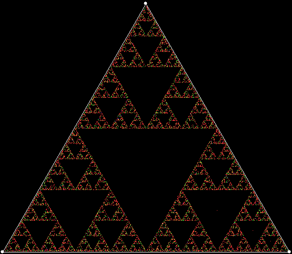
Sierpiński triangle from point jumping halfway to randomly chosen vertex

Sierpiński pentagon from point jumping halfway to randomly chosen vertex
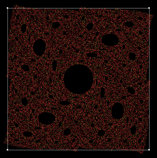
But it doesn’t work with a square. Instead, the interior of the square slowly fills with random points:

Square filling with point jumping halfway to randomly chosen vertex
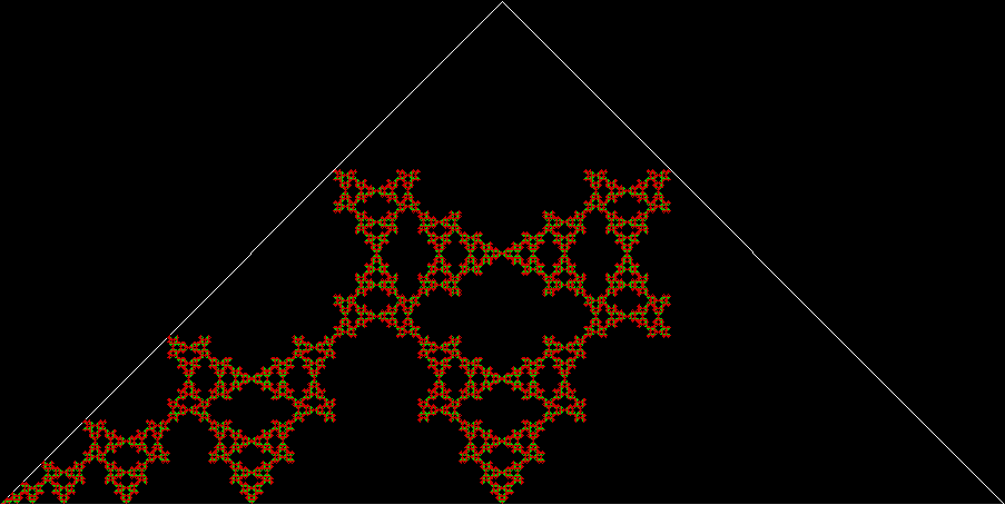
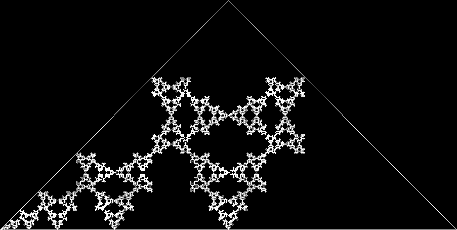
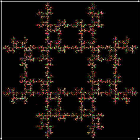
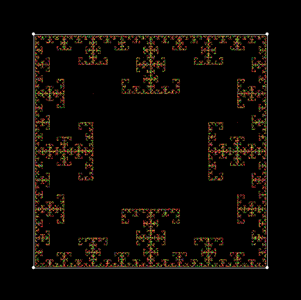
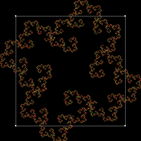
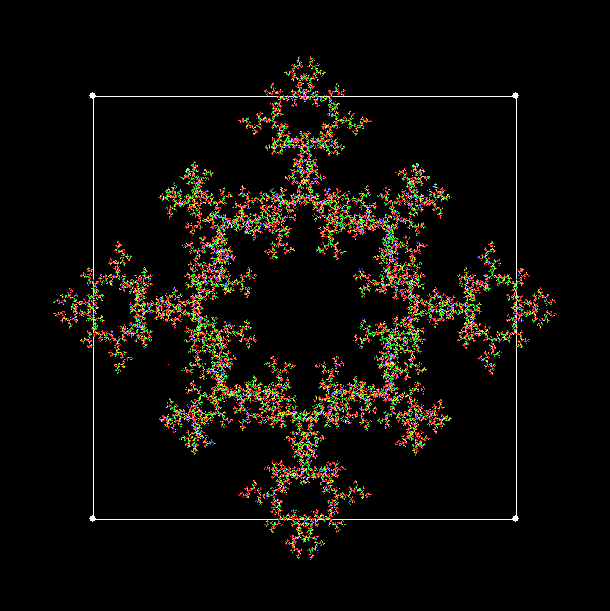
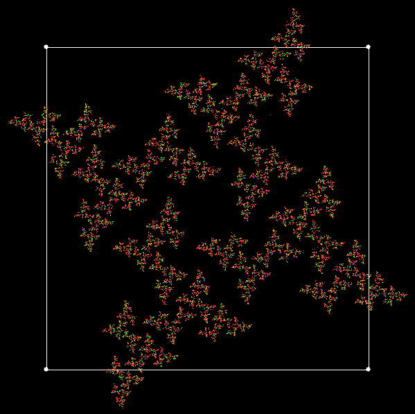
As I showed in Polymorphous Perverticity, you can create fractals from squares and randomly moving points if you ban the point from choosing the same vertex twice in a row, and so on. But there are other ways. You can take the point, move it towards a vertex at random, then swing it around the center of the square through some angle before you mark its position, like this:

Point moves at random, then swings by 90° around center

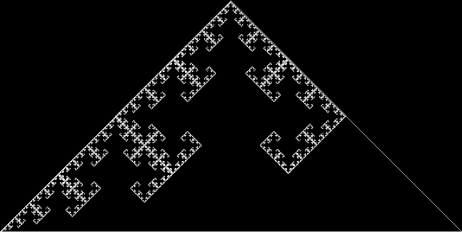
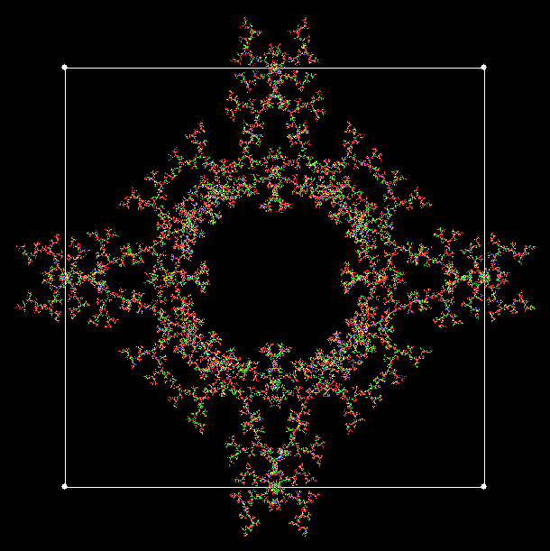
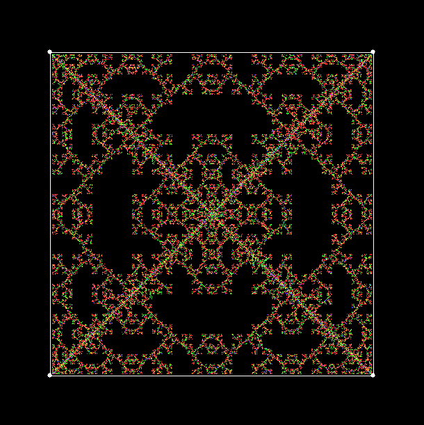
Point moves at random, then swings by 180° around center
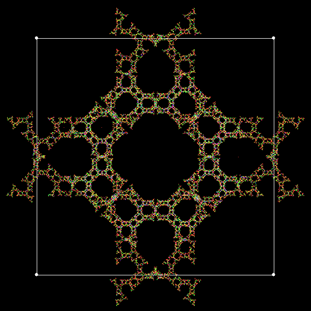
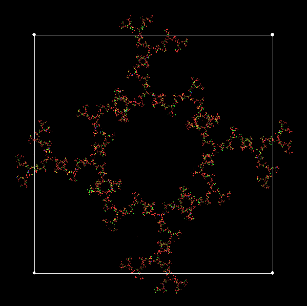
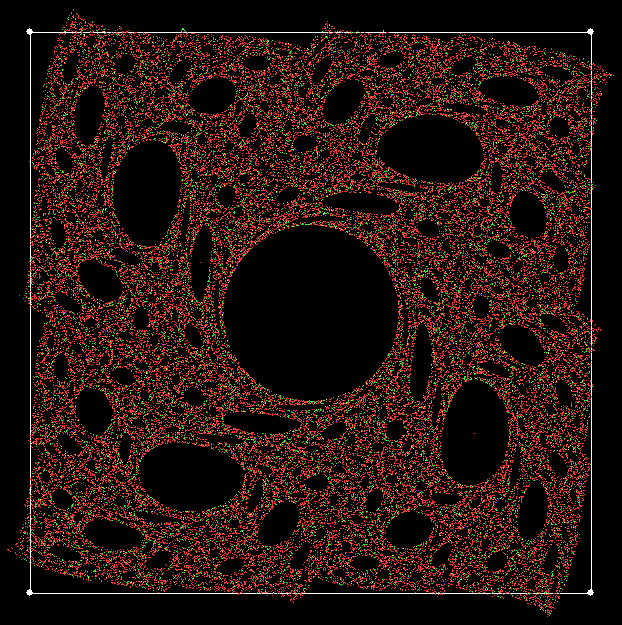
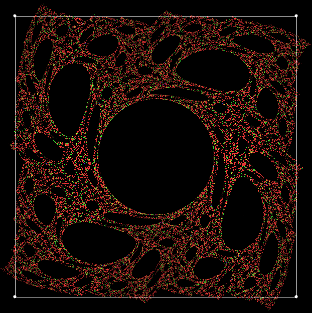
You can also adjust the distance of the point from the center of the square using a formula like dist = r * rm – dist, where dist is the distance, r is the radius of the circle in which the circle is drawn, and rm takes values like 0.1, 0.25, 0.5, 0.75 and so on:

Point moves at random, dist = r * 0.05 – dist

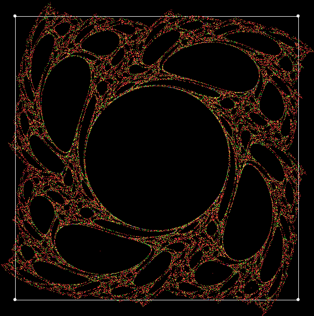
Point moves at random, dist = r * 0.1 – dist

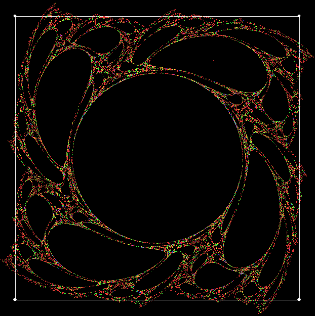
Point moves at random, dist = r * 0.2 – dist
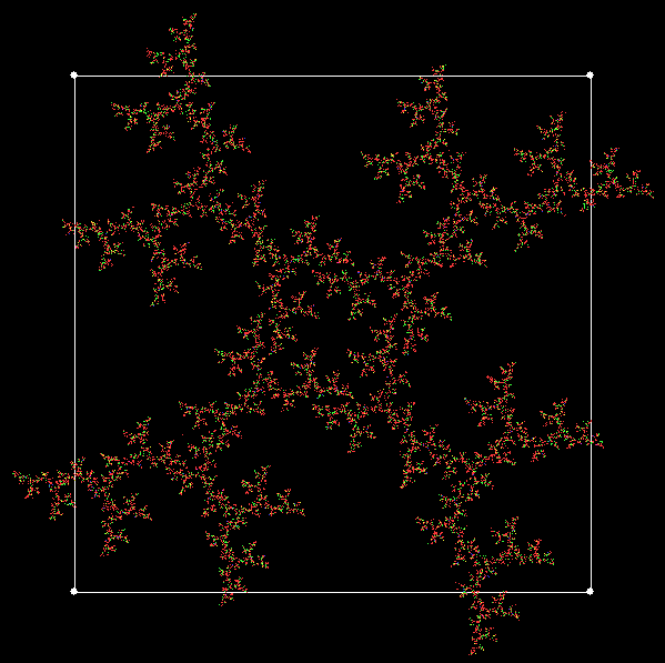
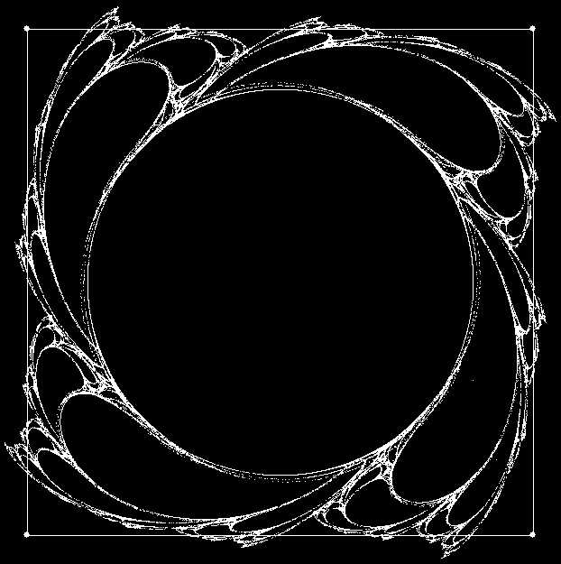
But you can swing the point while applying a vertex-ban, like banning the previously chosen vertex, or the vertex 90° or 180° away. In fact, swinging the points converts one kind of vertex ban into the others.
Point moves at random towards vertex not chosen previously
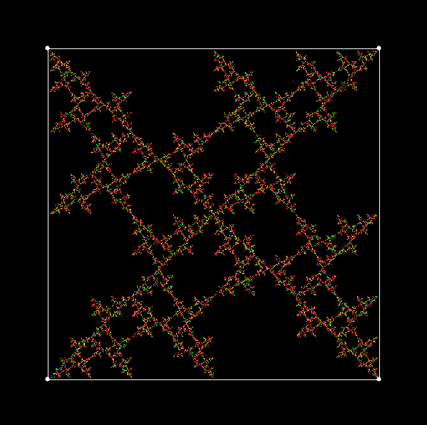
Point moves at random, then swings by 45°
Point moves at random, then swings by 360°
Point moves at random, then swings by 697.5°
Point moves at random, then swings by 720°
Point moves at random, then swings by 652.5°
Animated angle swing
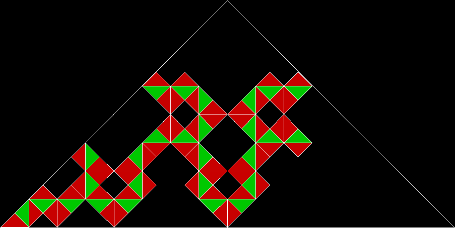
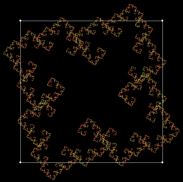
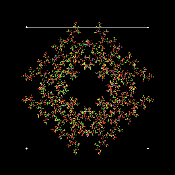
You can also reverse the swing at every second move, swing the point around a vertex instead of the center or around a point on the circle that encloses the square. Here are some of the fractals you get applying these techniques.
Point moves at random, then swings alternately by 45°, -45°
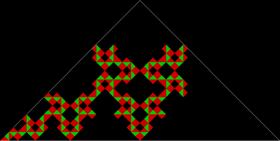
Point moves at random, then swings alternately by 90°, -90°
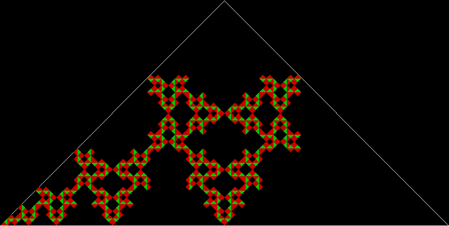
Point moves at random, then swings alternately by 135°, -135°
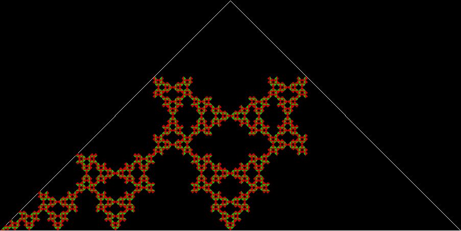
Point moves at random, then swings alternately by 180°, -180°
Point moves at random, then swings alternately by 225°, -225°
Point moves at random, then swings alternately by 315°, -315°
Point moves at random, then swings alternately by 360°, -360°

Animated alternate swing
Point moves at random, then swings around point on circle by 45°
Point moves at random, then swings around point on circle by 67.5°
Point moves at random, then swings around point on circle by 90°
Point moves at random, then swings around point on circle by 112.5°
Point moves at random, then swings around point on circle by 135°
Point moves at random, then swings around point on circle by 180°
Animated circle swing