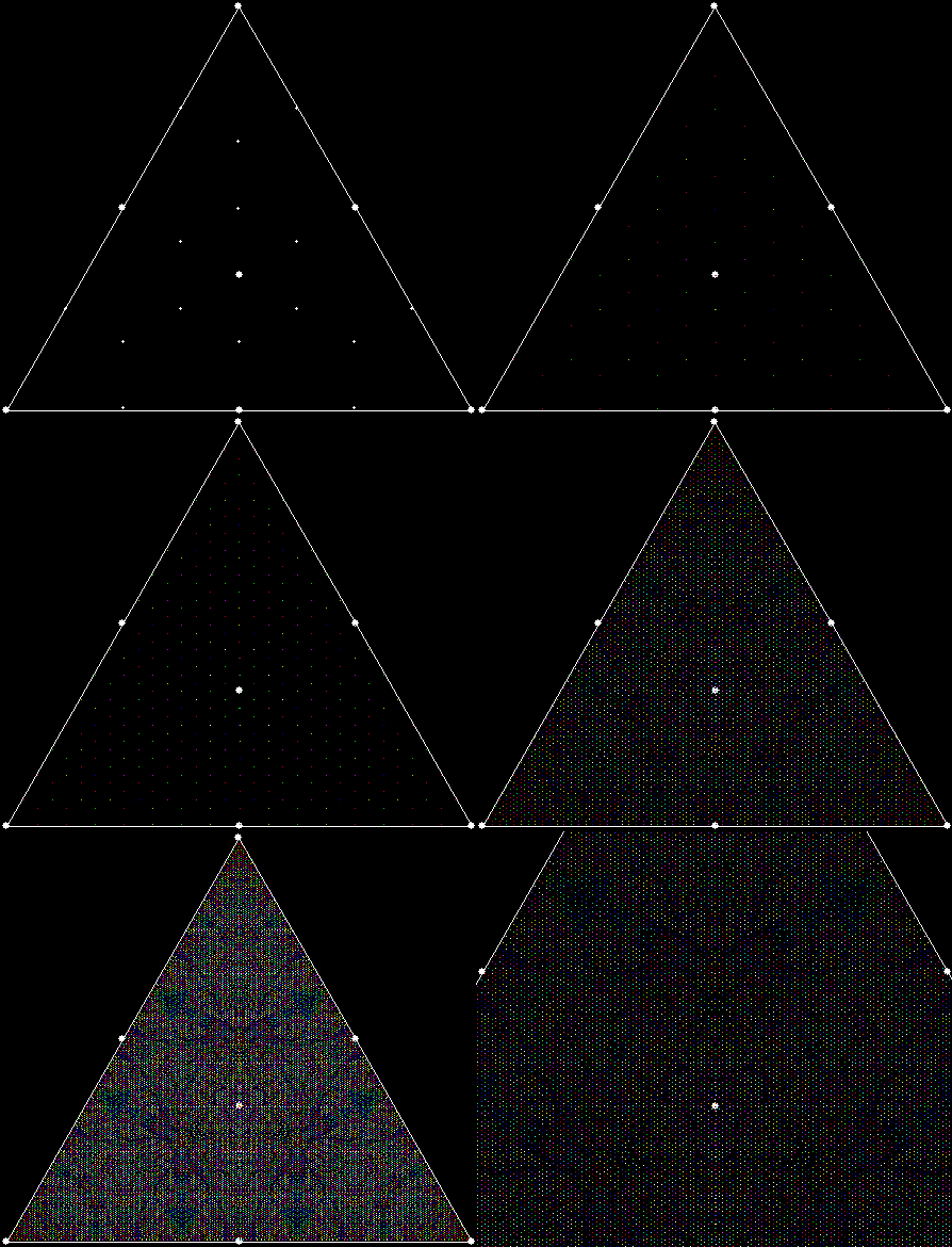
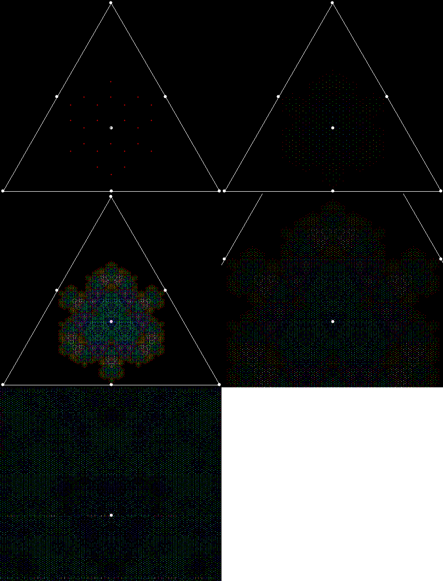
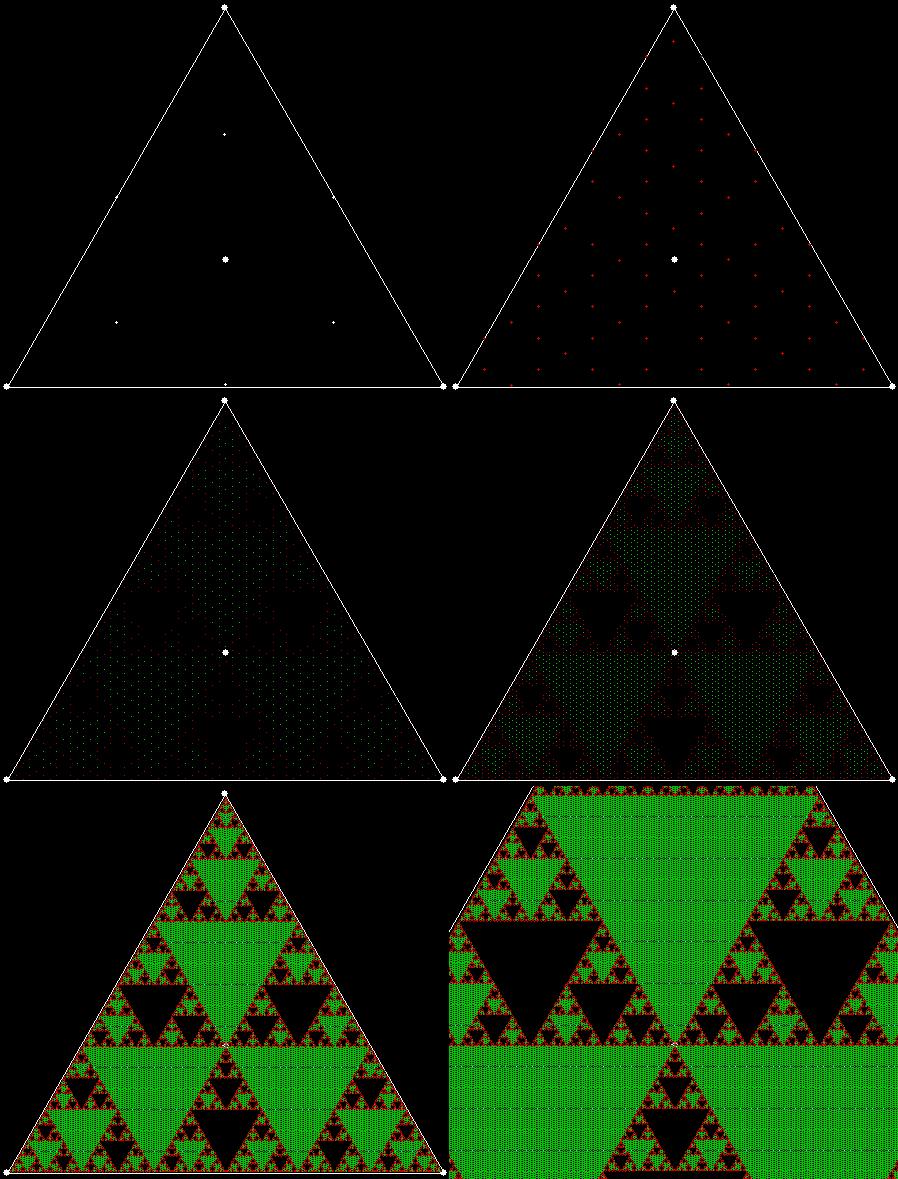
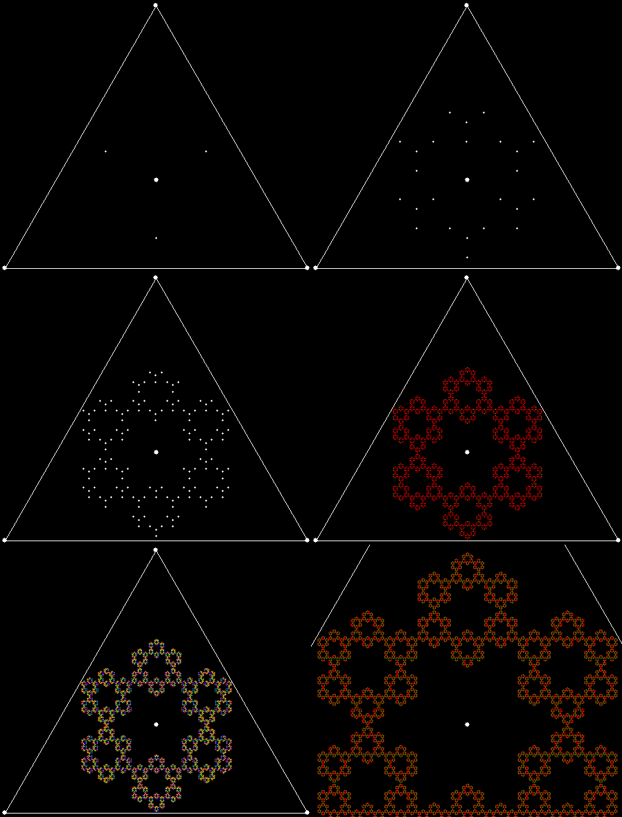
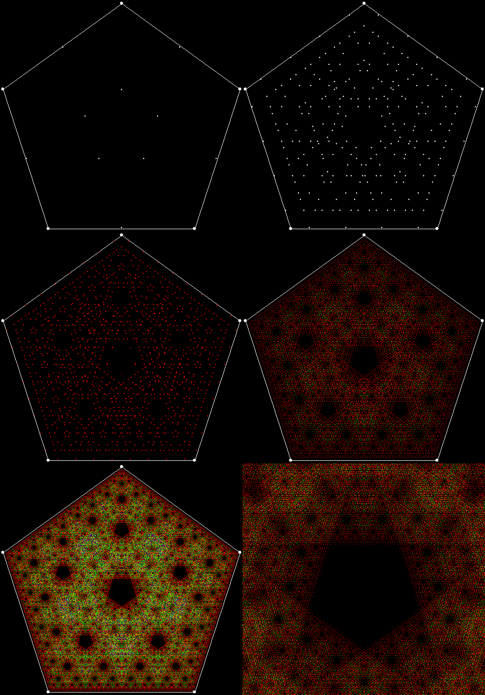
De Pluribus Unum

A beautifully subtle puzzle:

Scrambled Box Tops

Imagine you have three boxes, one containing two black marbles, one containing two white marbles, and the third, one black and one white marble. The boxes are labelled according to their contents — BB, WW, and BW — but someone has switched the labels so that every box is now incorrectly labelled. You are allowed to take one marble at a time out of any box, without looking inside, and by this process of sampling you are to determine the contents of all three boxes. What is the smallest number of drawings needed to do this? — Martin Gardner, Mathematical Puzzles and Diversions (1959), chapter 3, “Nine Problems”, #5.

Bald eagle, Haliaeetus leucocephalus (Linnaeus 1776)

Bald eagle, Haliaeetus leucocephalus (Linnaeus 1776)

Answer: You can learn the contents of all three boxes by drawing just one marble. The key to the solution is your knowledge that the labels on all three boxes are incorrect. You must draw a marble from the box labelled “black-white”. Assume that the marble drawn is black. You know then that the other marble in the box must be black also, otherwise the label on the box would be correct. Since you have now identified the box containing two black marbles, you can tell at once the contents of the box labelled “white-white”: you know it cannot contain two white marbles, because its label has to be wrong; it cannot contain two black marbles, because you have identified that box; therefore it must contain one black and one white marble. The third box, of course, must then be the one containing two white marbles. You can solve the puzzle by the same reasoning if the marble you draw from the “black-white” box happens to be white instead of black.

For Revver and Fevver

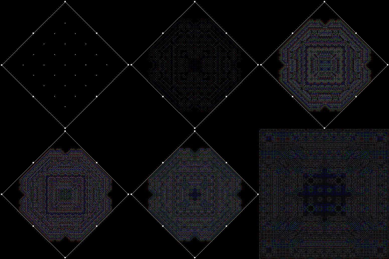
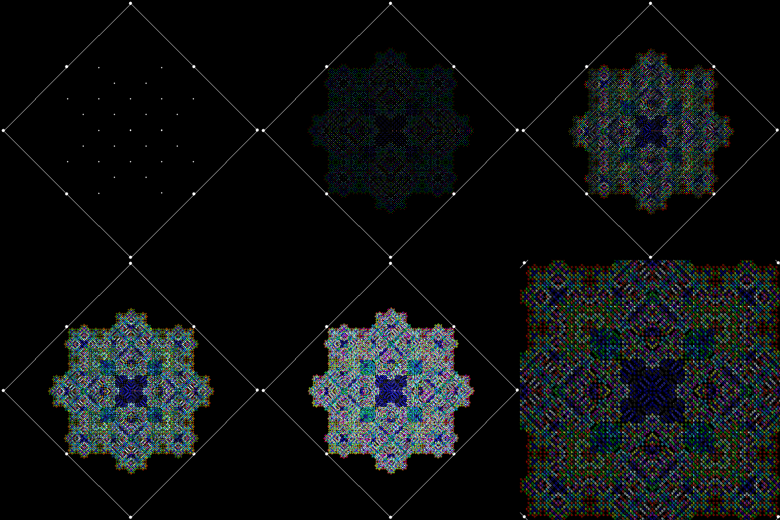
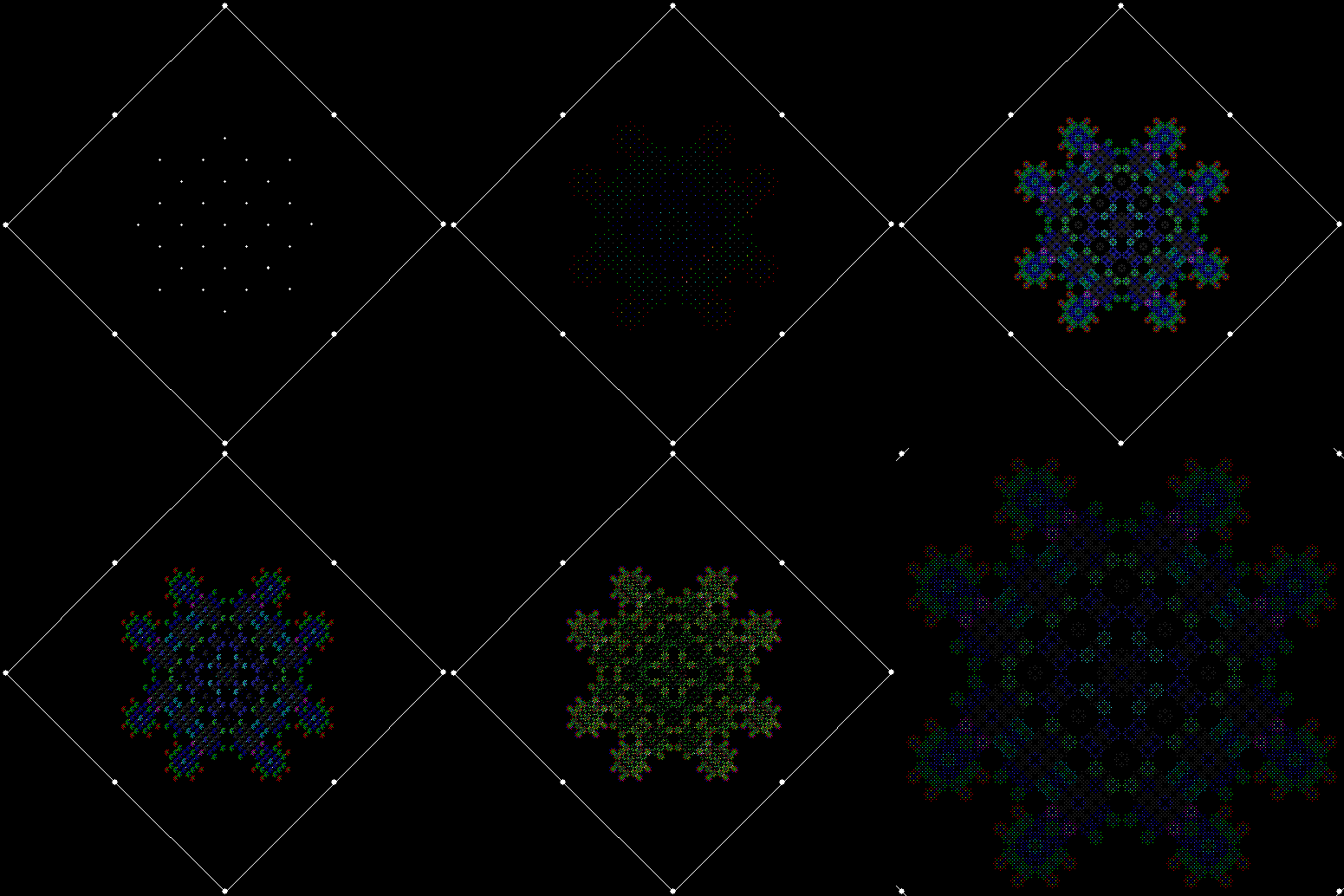
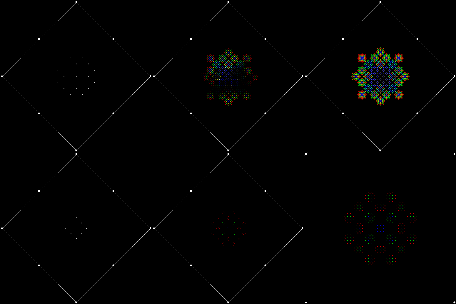
This shape reminds me of the feathers on an exotic bird:

feathers

(click or open in new window for full size)


feathers_anim

(animated version)


The shape is created by reversing the digits of a number, so you could say it involves revvers and fevvers. I discovered it when I was looking at the Halton sequence. It’s a sequence of fractions created according to a simple but interesting rule. The rule works like this: take n in base b, reverse it, and divide reverse(n) by the first power of b that is greater than n.

For example, suppose n = 6 and b = 2. In base 2, 6 = 110 and reverse(110) = 011 = 11 = 3. The first power of 2 that is greater than 6 is 2^3 or 8. Therefore, halton(6) in base 2 equals 3/8. Here is the same procedure applied to n = 1..20:

1: halton(1) = 1/10[2] → 1/2
2: halton(10) = 01/100[2] → 1/4
3: halton(11) = 11/100[2] → 3/4
4: halton(100) = 001/1000[2] → 1/8
5: halton(101) = 101/1000[2] → 5/8
6: halton(110) = 011/1000 → 3/8
7: halton(111) = 111/1000 → 7/8
8: halton(1000) = 0001/10000 → 1/16
9: halton(1001) = 1001/10000 → 9/16
10: halton(1010) = 0101/10000 → 5/16
11: halton(1011) = 1101/10000 → 13/16
12: halton(1100) = 0011/10000 → 3/16
13: halton(1101) = 1011/10000 → 11/16
14: halton(1110) = 0111/10000 → 7/16
15: halton(1111) = 1111/10000 → 15/16
16: halton(10000) = 00001/100000 → 1/32
17: halton(10001) = 10001/100000 → 17/32
18: halton(10010) = 01001/100000 → 9/32
19: halton(10011) = 11001/100000 → 25/32
20: halton(10100) = 00101/100000 → 5/32…

Note that the sequence always produces reduced fractions, i.e. fractions in their lowest possible terms. Once 1/2 has appeared, there is no 2/4, 4/8, 8/16…; once 3/4 has appeared, there is no 6/8, 12/16, 24/32…; and so on. If the fractions are represented as points in the interval [0,1], they look like this:

line1_1_2

point = 1/2


line2_1_4

point = 1/4


line3_3_4

point = 3/4


line4_1_8

point = 1/8


line5_5_8

point = 5/8


line6_3_8

point = 3/8


line7_7_8

point = 7/8


line_b2_anim

(animated line for base = 2, n = 1..63)


It’s apparent that Halton points in base 2 will evenly fill the interval [0,1]. Now compare a Halton sequence in base 3:

1: halton(1) = 1/10[3] → 1/3
2: halton(2) = 2/10[3] → 2/3
3: halton(10) = 01/100[3] → 1/9
4: halton(11) = 11/100[3] → 4/9
5: halton(12) = 21/100[3] → 7/9
6: halton(20) = 02/100 → 2/9
7: halton(21) = 12/100 → 5/9
8: halton(22) = 22/100 → 8/9
9: halton(100) = 001/1000 → 1/27
10: halton(101) = 101/1000 → 10/27
11: halton(102) = 201/1000 → 19/27
12: halton(110) = 011/1000 → 4/27
13: halton(111) = 111/1000 → 13/27
14: halton(112) = 211/1000 → 22/27
15: halton(120) = 021/1000 → 7/27
16: halton(121) = 121/1000 → 16/27
17: halton(122) = 221/1000 → 25/27
18: halton(200) = 002/1000 → 2/27
19: halton(201) = 102/1000 → 11/27
20: halton(202) = 202/1000 → 20/27
21: halton(210) = 012/1000 → 5/27
22: halton(211) = 112/1000 → 14/27
23: halton(212) = 212/1000 → 23/27
24: halton(220) = 022/1000 → 8/27
25: halton(221) = 122/1000 → 17/27
26: halton(222) = 222/1000 → 26/27
27: halton(1000) = 0001/10000 → 1/81
28: halton(1001) = 1001/10000 → 28/81
29: halton(1002) = 2001/10000 → 55/81
30: halton(1010) = 0101/10000 → 10/81

And here is an animated gif representing the Halton sequence in base 3 as points in the interval [0,1]:

line_b3_anim


Halton points in base 3 also evenly fill the interval [0,1]. What happens if you apply the Halton sequence to a two-dimensional square rather a one-dimensional line? Suppose the bottom left-hand corner of the square has the co-ordinates (0,0) and the top right-hand corner has the co-ordinates (1,1). Find points (x,y) inside the square, with x supplied by the Halton sequence in base 2 and y supplied by the Halton sequence in base 3. The square will gradually fill like this:

square1

x = 1/2, y = 1/3


square2

x = 1/4, y = 2/3


square3

x = 3/4, y = 1/9


square4

x = 1/8, y = 4/9


square5

x = 5/8, y = 7/9


square6

x = 3/8, y = 2/9


square7

x = 7/8, y = 5/9


square8

x = 1/16, y = 8/9


square9

x = 9/16, y = 1/27…


square_anim

animated square


Read full page: For Revver and Fevver

Pigmental Paradox

From Raymond Smullyan’s Logical Labyrinths (2009):

We now visit another knight/knave island on which, like on the first one, all knights tell the truth and all knaves lie. But now there is another complication! For some reason, the natives refuse to speak to strangers, but they are willing to answer yes/no questions using a secret sign language that works like this:

Each native carries two cards on his person; one is red and the other is black. One of them means yes and the other means no, but you are not told which color means what. If you ask a yes/no question, the native will flash one of the two cards, but unfortunately, you will not know whether the card means yes or no!

Problem 3.1. Abercrombie, who knew the rules of this island, decided to pay it a visit. He met a native and asked him: “Does a red card signify yes?” The native then showed him a red card.

From this, is it possible to deduce what a red card signifies? Is it possible to deduce whether the native was a knight or a knave?

Problem 3.2. Suppose one wishes to find out whether it is a red card or a black card that signifies yes. What simple yes/no question should one ask?

Fragic Carpet

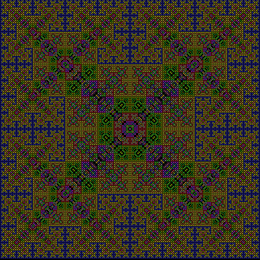
Maths is like a jungle: rich, teeming and full of surprises. A waterfall here, a glade of butterflies there, a bank of orchids yonder. There is always something new to see and a different route to try. But sometimes a different route will take you to the same place. I’ve already found two ways to reach this fractal (see Fingering the Frigit and Performativizing the Polygonic):

carpet2x2

Fractal Carpet


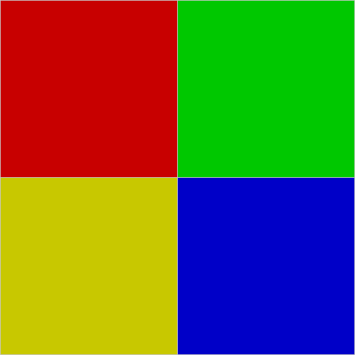
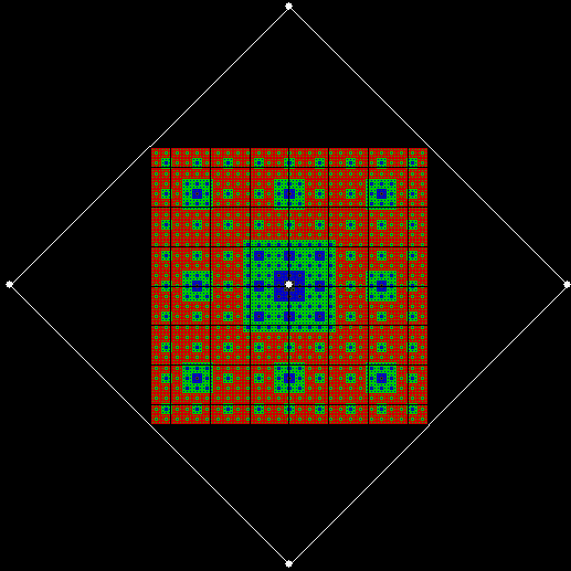
Now I’ve found a third way. You could call it the rep-tile route. Divide a square into four smaller squares:

square2x2

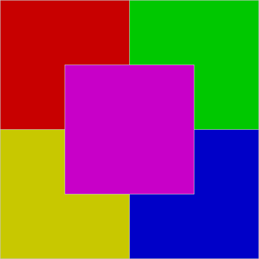
Add an extra square over the centre:

square2x2_1

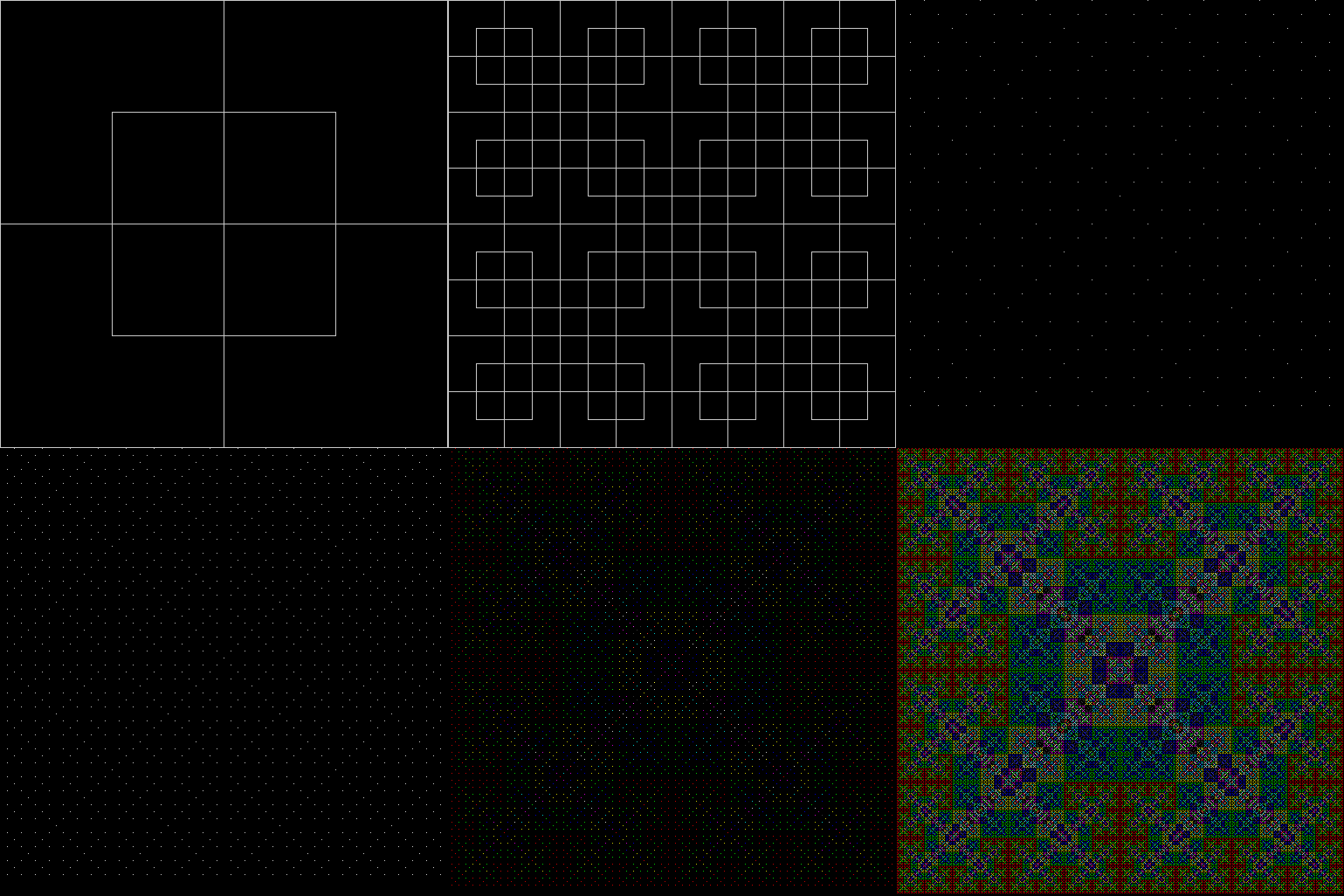
Then keep dividing the squares in the same way:

carpet2x2_anim_1

Animated carpet (with coloured blocks)


carpet2x2_anim_2

Animated carpet (with empty blocks)


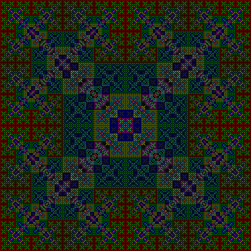
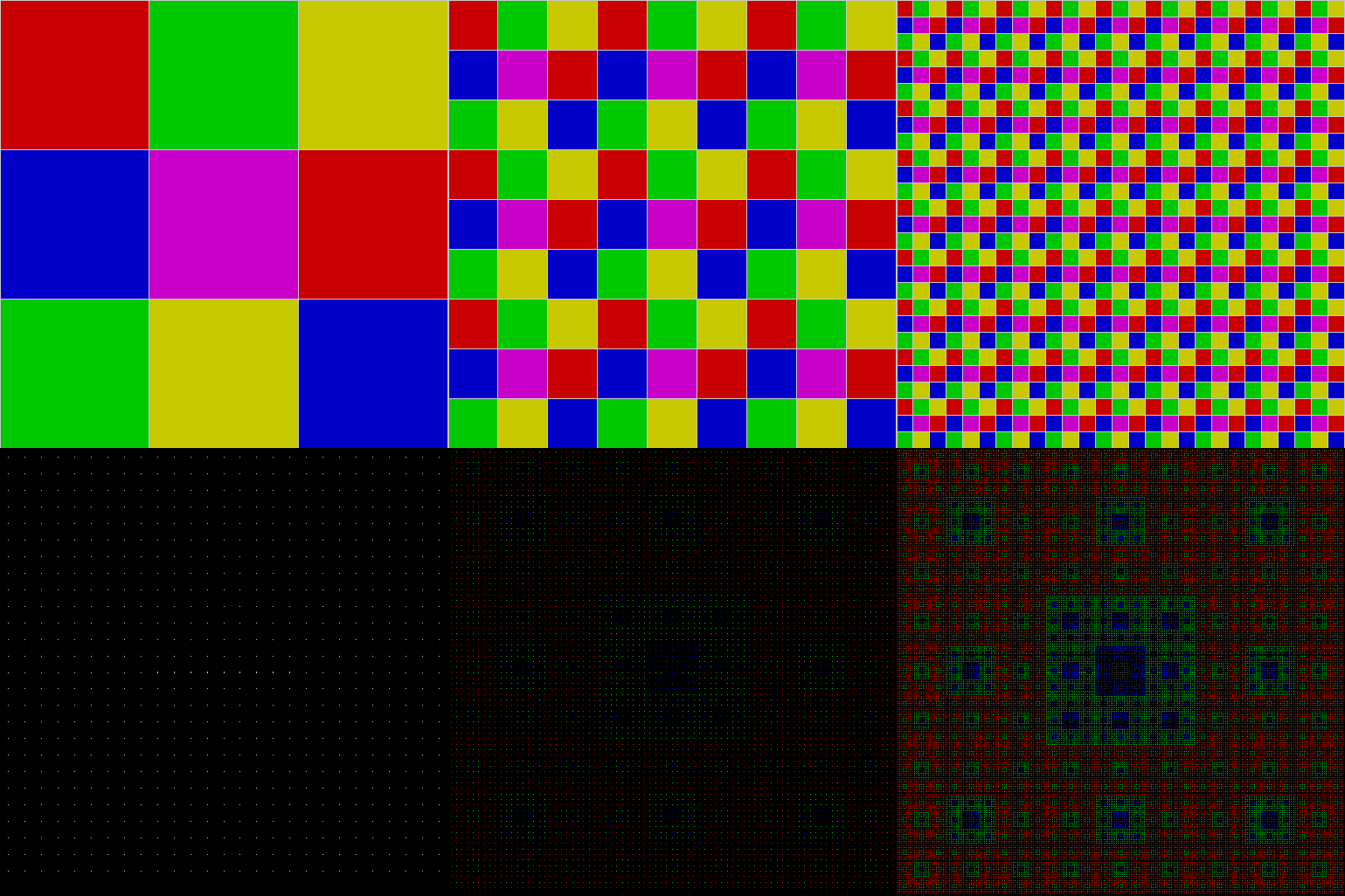
The colours of the fractal appear when the same pixel is covered repeatedly: first it’s red, then green, yellow, blue, purple, and so on. Because the colours and their order are arbitrary, you can use different colour schemes:

carpet2x2_col1

Colour scheme #1


carpet2x2_col2

Colour scheme #2


carpet2x2_col3

Colour scheme #3


Here are more colour-schemes in an animated gif:

carpet2x2_col

Various colour-schemes


Now try dividing the square into nine and sixteen, with an extra square over the centre:

carpet3x3

3×3 square + central square


carpet3x3_anim

3×3 square + central square (animated)


carpet4x4

4×4 square + central square


carpet4x4_anim

4×4 square + central square (animated)


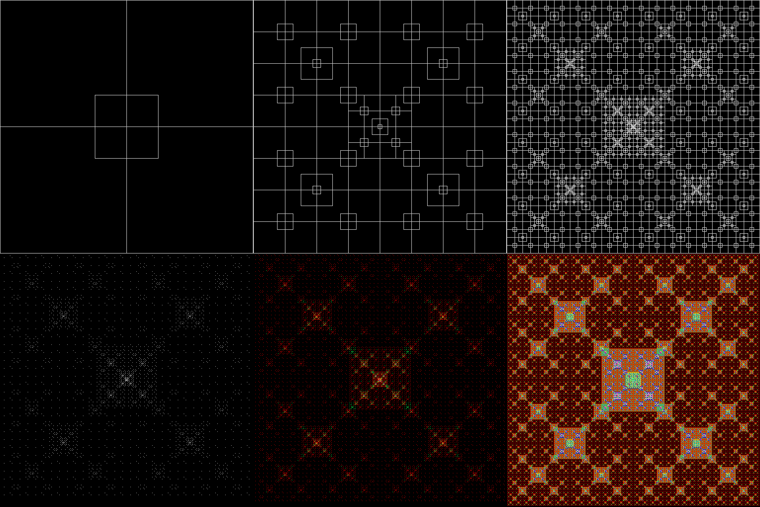
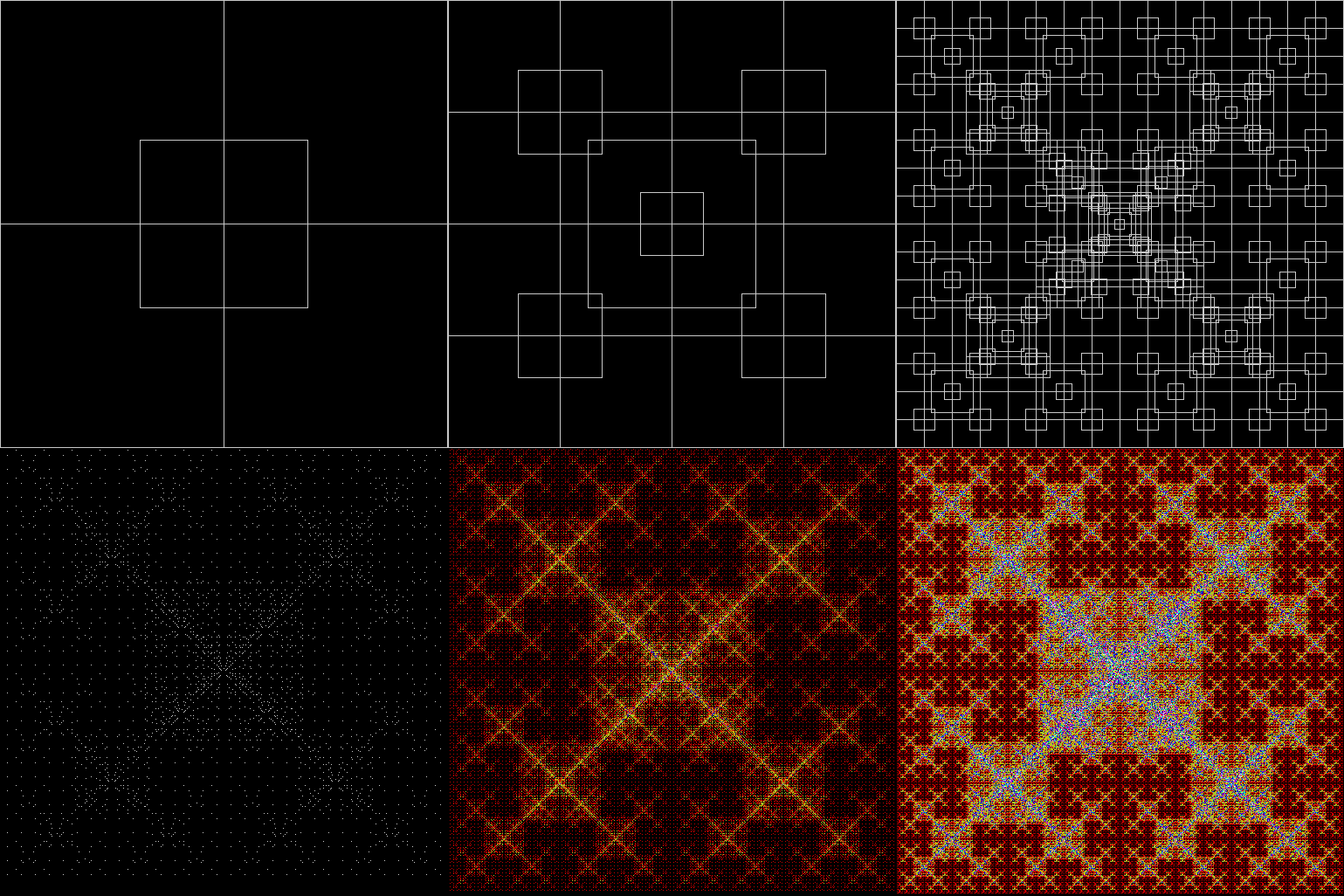
You can also adjust the size of the square added to the 2×2 subdivision:

carpet2x2_1_2

2×2 square + 1/2-sized central square


carpet2x2_3_4

2×2 square + 3/4-sized central square


Elsewhere Other-Posted:

Fingering the Frigit
Performativizing the Polygonic

Polymorphous Pursuit

Suppose four mice are standing on the corners of a large square. Each mouse begins running at the same speed towards the mouse one place away, reckoning clockwise. The mice will meet at the centre of the square and the path taken by each mouse will be what is known as a pursuit curve:

v4_mi1

vertices = 4, mouse-increment = 1


v4_mi1_animated

v = 4, mi = 1 (animated)


As I showed in “Persecution Complex”, it’s easy to find variants on the basic pursuit curve. If mi = 2, i.e. each mouse runs towards the mouse two places away, the mice will run in straight lines direct to the centre of the square:

v4_mi2

v = 4, mi = 2


v4_mi2_animated

v = 4, mi = 2 (animated)


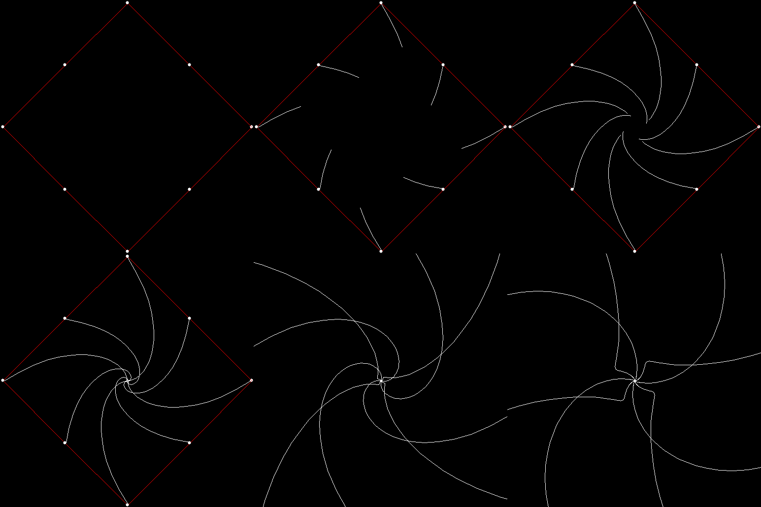
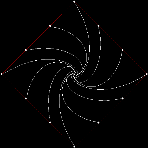
That variant is trivial, but suppose there are eight mice, four starting on the corners of the square and four starting on the midpoints of the sides. Mice starting on the corners will run different pursuit curves to those starting on the midpoints, because the corners are further from the centre than the midpoints are:

v4_si1_mi1

v = 4, si = 1, mi = 1


v4_si1_mi1_extra


If mi = 3, the pursuit curves look like this:

v4_si1_mi3

v = 4, si = 1, mi = 3


v4_si1_mi3_animated

v = 4, si = 1, mi = 3 (animated)


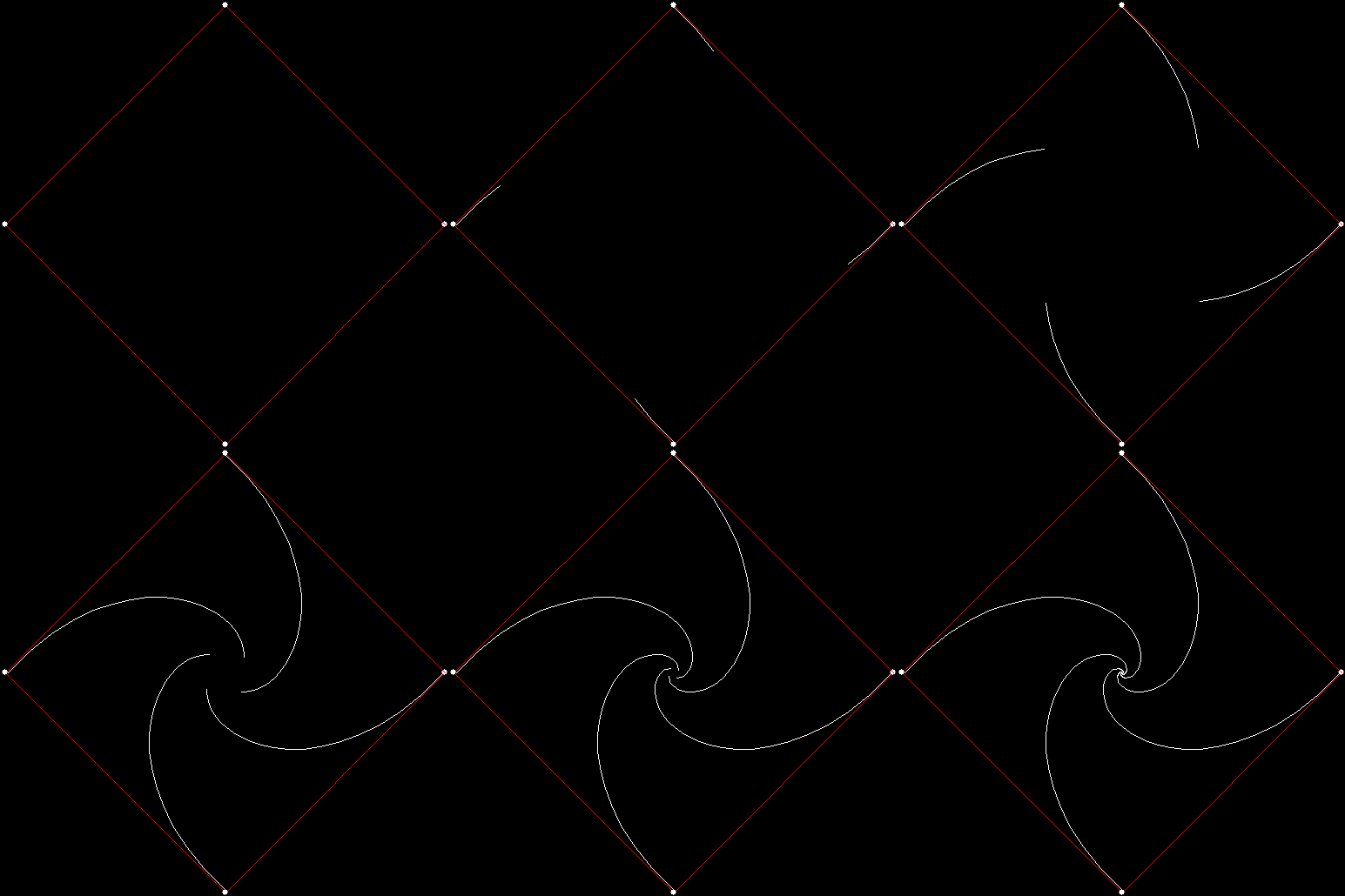
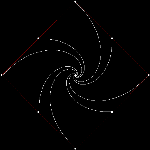
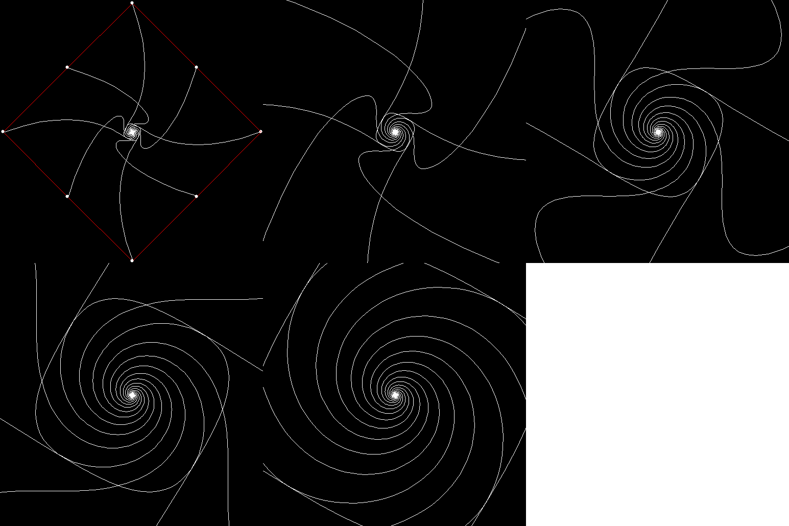
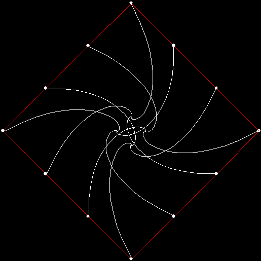
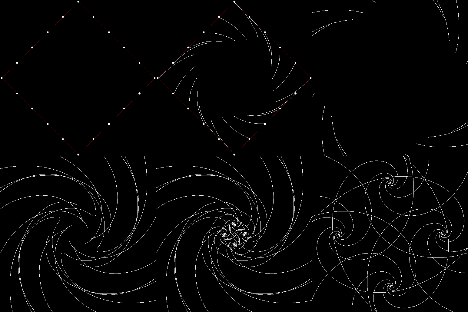
Suppose there are twelve mice, four on each corner and two more on each side. If each mouse runs towards the mouse four places away, then the pursuit curves don’t all meet in the centre of the square. Instead, they meet in groups of three at four points equidistant from the centre, like this:

v4_si2_mi4

v4_si2_mi4_curves

v = 4, si = 2, mi = 4


v4_si2_mi4_animated

v = 4, si = 2, mi = 4 (animated)


v4_si4_mi4_animated

v = 4, si = 4, mi = 4 (animated)


v4_si4_mi4_large

v = 4, si = 4, mi = 4 (zoom)


Now suppose each mouse become sophisticated and runs toward the combined positions of two other mice, one two places away, the other three places away, like this:

v4_si1_mi2_3

v = 4, si = 1, mi = (2, 3)


v4_si1_mi2_3_animated

v = 4, si = 1, mi = (2, 3) (animated)


These polypursuits, as they could be called, can have complicated central regions:

v4_si2_mi1_4

v = 4, si = 2, mi = (1, 4)


v4_si2_mi1_4_animated

v = 4, si = 2, mi = (1, 4) (animated)


v4_si_va_mi_va

v = 4, si = various, mi = various


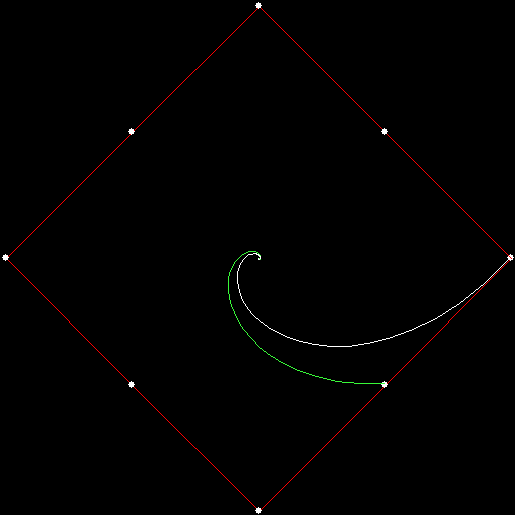
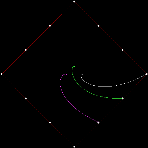
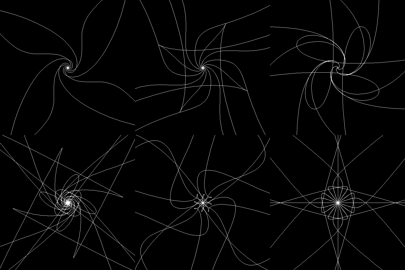
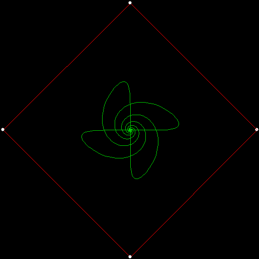
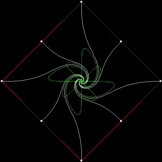
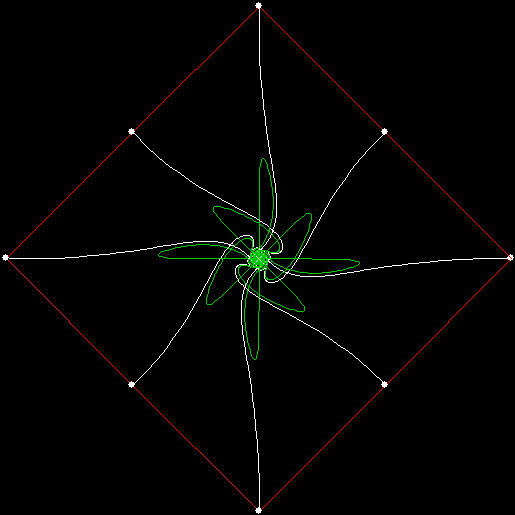
And what if you have two teams of mice, running towards one or more mice on the other team? For example, suppose two mice, one from each team, start on each corner of a square. Each mouse on team 1 runs towards the mouse on team 2 that is one place away, while each mouse on team 2 runs towards the mouse on team 1 that is two places away. If the pursuits curves of team 1 are represented in white and the pursuit curves of team 2 in green, the curves look like this:

2v4_mi1_mi2

v = 4 * 2, vmi = 1, vmi = 2


2v4_mi1_mi2_green

v = 4 * 2, vmi = 1, vmi = 2


2v4_mi1_mi2_animated

v = 4 * 2, vmi = 1, vmi = 2 (animated)


Now suppose the four mice of team 1 start on the corners while the mice of team 2 start at the centre of the square.

v4_c4_vmi1_cmi2_white

v = 4, centre = 4, vmi = 1, cmi = 2 (white team)


v4_c4_vmi1_cmi2_green

v = 4, centre = 4, vmi = 1, cmi = 2 (green team)


v4_c4_vmi1_cmi2_both

v = 4, centre = 4, vmi = 1, cmi = 2 (both teams)


v4_c4_vmi1_cmi2_animated

v = 4, centre = 4, vmi = 1, cmi = 2 (animated)


Here are more variants on pursuit curves formed by two teams of mice, one starting on the corners, one at the centre:

v4_c4_vmi0_1_cmi0

v = 4, centre = 4, vmi = (0, 1), cmi = 0


v4_c4_vmi0_2_cmi0

v = 4, centre = 4, vmi = (0, 2), cmi = 0


v4_c4_vmi0_3_cmi0

v = 4, centre = 4, vmi = (0, 3), cmi = 0


2v4_mi1_mi2_both

White Rites

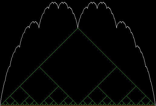
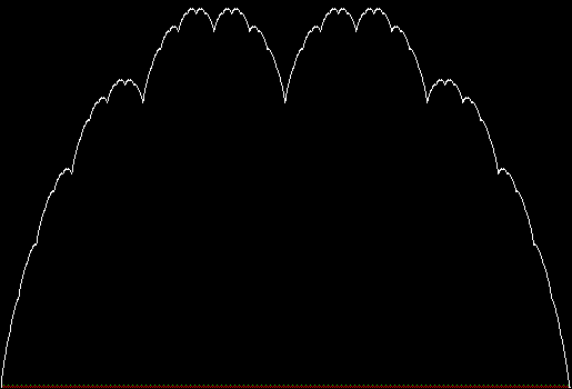
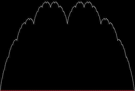
The blancmange curve is an interesting fractal formed by summing a series of zigzags. It
takes its name from its resemblance to the milk-pudding known as a blancmange
(blanc-manger in French, meaning “white eating”):

blanc_solid

Blancmange curve


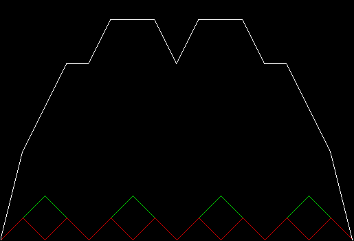
In successive zigzags, the number of zags doubles as their height halves, i.e. z(i) = z(i-1) * 2, h(i) = h(i-1) / 2. If all the zigzags are represented at once, the construction looks like this:

blanc_all

Zigzags 1 to 10


blancmange_all

Zigzags 1 to 10 (animated)


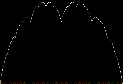
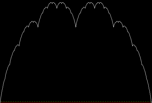
Here is a step-by-step construction, with the total sum of zigzags in white, the present zigzag in red and the previous zigzag in green:

blanc1

Blancmange curve stage 1


blanc2

Stage 2


blanc3

Stage 3


blanc4

Stage 4


blanc5

Stage 5


blanc6

Stage 6


blanc7

Stage 7


blanc8

Stage 8


blanc9

Stage 9


blanc10

Stage 10


blancmange

Blancmange curve (animated)


It’s easy to think of variants on the standard blancmange curve. Suppose the number of zags triples as their height is divided by three, i.e. z(i) = z(i-1) * 3, h(i) = h(i-1) / 3:

blanc_x3_solid

Blancmange curve for z(i) = z(i-1) * 3, h(i) = h(i-1) / 3


Continue reading “White Rites”…

Get Your Ox Off

Boustrophedon (pronounced “bough-stra-FEE-dun” or “boo-stra-FEE-dun”) is an ancient Greek word literally meaning “as the ox turns (in ploughing)”, that is, moving left-right, right-left, and so on. The word is used of writing that runs down the page in the same way. To see what that means, examine two versions of the first paragraph of Clark Ashton Smith’s story “The Demon of the Flower” (1933). The first is written in the usual way, the second is written boustrophedon:

Not as the plants and flowers of Earth, growing peacefully beneath a simple sun, were the blossoms of the planet Lophai. Coiling and uncoiling in double dawns; tossing tumultuously under vast suns of jade green and balas-ruby orange; swaying and weltering in rich twilights, in aurora-curtained nights, they resembled fields of rooted servants that dance eternally to an other-worldly music.


Not as the plants and flowers of Earth, growing peacefully
.iahpoL tenalp eht fo smossolb eht erew ,nus elpmis a htaeneb
Coiling and uncoiling in double dawns; tossing tumultuously
;egnaro ybur-salab dna neerg edaj fo snus tsav rednu
swaying and weltering in rich twilights, in aurora-curtained
ecnad taht stnavres detoor fo sdleif delbmeser yeht ,sthgin
eternally to an other-worldly music.


Boustrophedon writing was once common and sometimes the left-right lines would also be mirror-reversed, like this:


You could also use the term “boustrophedon” to describe the way this table of numbers is filled:

primes_table


The table begins with “1” in the top left-hand corner, then moves right for “2”, then down for “3”, then right-and-up for “4”, “5” and “6”, then right for “7”, then left-and-down for “8”, “9” and “10”, and so on. You could also say that the numbers snake through the table. I’ve marked the primes among them, because I was interested in the patterns made by the primes when the numbers were represented as blocks on a grid, like this:

primes_large


Primes are in solid white (compare the Ulam spiral). Here’s the boustrophedon prime-grid on a finer scale:

primes

(click for full image)


And what about other number-tests? Here are the even numbers marked on the grid (i.e. n mod 2 = 0):

mod2

n mod 2 = 0


And here are some more examples of a modulus test:

mod3

n mod 3 = 0


mod5

n mod 5 = 0


mod9

n mod 9 = 0


mod15

n mod 15 = 0


mod_various

n mod various = 0 (animated gif)


Next I looked at reciprocals (numbers divided into 1) marked on the grid, with the digits of a reciprocal marking the number of blank squares before a square is filled in (if the digit is “0”, the square is filled immediately). For example, in base ten 1/7 = 0.142857142857142857…, where the block “142857” repeats for ever. When represented on the grid, 1/7 has 1 blank square, then a filled square, then 4 blank squares, then a filled square, then 2 blank squares, then a filled square, and so on:

recip7_base10

1/7 in base 10


And here are some more reciprocals (click for full images):

recip9_base2

1/9 in base 2


recip13_base10

1/13 in base 10


recip27_base10

1/27 in base 10


recip41_base10

1/41 in base 10


recip63_base10

1/63 in base 10


recip82_base10

1/82 in base 10


recip101_base10

1/101 in base 10


recip104_base10

1/104 in base 10


recip124_base10

1/124 in base 10


recip143_base10

1/143 in base 10


recip175_base10

1/175 in base 10


recip604_base8

1/604 in base 8


recip_various

1/n in various bases (animated gif)


Get Your Prox Off #2

Serendipity is the art of making happy discoveries by accident. I made a mistake writing a program to create fractals and made the happy discovery of an attractive new fractal. And also of a new version of an attractive fractal I had seen before.

As I described in Get Your Prox Off, you can create a fractal by 1) moving a point towards a randomly chosen vertex of a polygon, but 2) forbidding a move towards the nearest vertex or the second-nearest vertex or third-nearest, and so on. If the polygon is a square, the four possible basic fractals look like this (note that the first fractal is also produced by banning a move towards a vertex that was chosen in the previous move):

v4_ban1

v = 4, ban = prox(1)
(ban move towards nearest vertex)
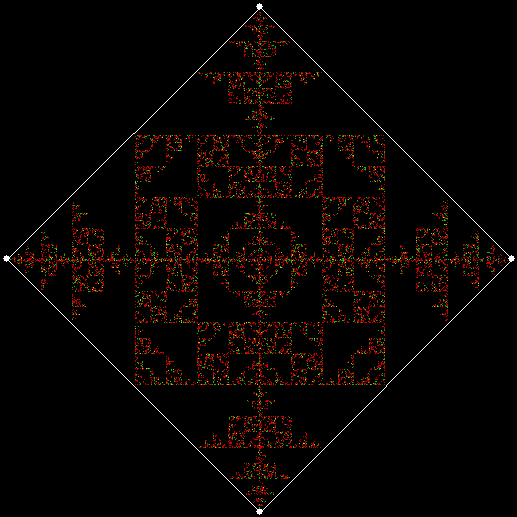

v4_ban2

v = 4, ban = prox(2)
(ban move towards second-nearest vertex)


v4_ban3

v = 4, ban = prox(3)


v4_ban4

v = 4, ban = prox(4)


This program has to calculate what might be called the order of proximity: that is, it creates an array of distances to each vertex, then sorts the array by increasing distance. I was using a bubble-sort, but made a mistake so that the program ran through the array only once and didn’t complete the sort. If this happens, the fractals look like this (note that vertex 1 is on the right, with vertex 2, 3 and 4 clockwise from it):
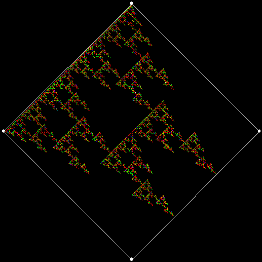
v4_ban1_sw1

v = 4, ban = prox(1), sweep = 1


v4_ban2_sw1

v = 4, ban = prox(2), sweep = 1


v4_ban3_sw1

v = 4, ban = prox(3), sweep = 1


v4_ban3_sw1_anim

(Animated version of v4, ban(prox(3)), sw=1)


v4_ban4_sw1

v = 4, ban = prox(4), sweep = 1


Note that in the last case, where ban = prox(4), a bubble-sort needs only one sweep to identify the most distant vertex, so the fractal looks the same as it does with a complete bubble-sort.

These new fractals looked interesting, so I had the idea of adjusting the number of sweeps in the incomplete bubble-sort: one sweep or two or three and so on (with enough sweeps, the bubble-sort becomes complete, but more sweeps are needed to complete a sort as the number of vertices increases). If there are two sweeps, then ban(prox(1)) and ban(prox(2)) look like this:
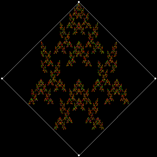
v4_ban1_sw2

v = 4, ban = prox(1), sweep = 2


v4_ban2_sw1

v = 4, ban = prox(2), sweep = 2


But the fractals produced by sweep = 2 for ban(prox(3)) and ban(prox(4)) are identical to the fractals produced by a complete bubble sort. Now, suppose you add a central point to the polygon and treat that as an additional vertex. If the bubble-sort is incomplete, a ban(prox(1)) fractal with a central point looks like this:
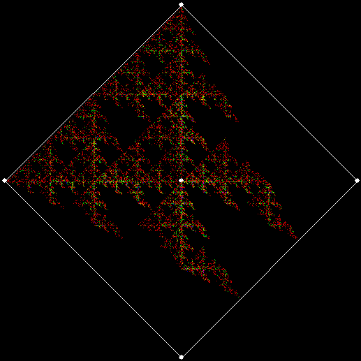
v4c_ban1_sw1

v = 4+c, ban = prox(1), sw = 1


v4c_ban1_sw2

v = 4+c, ban = prox(1), sw = 2


When sweep = 3, an attractive new fractal appears:
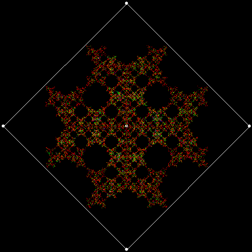
v4c_ban1_sw3

v = 4+c, ban = prox(1), sw = 3


v4c_ban1_sw3_anim

v = 4+c, ban = prox(1), sw = 3 (animated)


If you ban two vertices, the nearest and second-nearest, i.e. ban(prox(1), prox(2)), a complete bubble-sort produces a familiar fractal:

v4_ban12

v = 4+c, ban = prox(1), prox(2)


And here is ban(prox(2), prox(4)), with a complete bubble-sort:
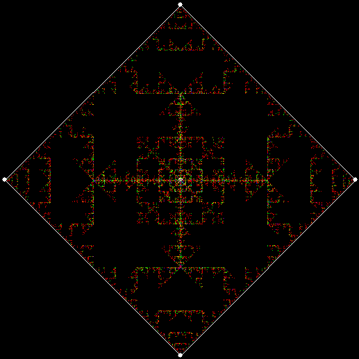
v4c_ban24

v = 4, ban = prox(2), prox(4)


If the bubble-sort is incomplete, sweep = 1 and sweep = 2 produce these fractals for ban(prox(1), prox(2)):

v4_ban12_sw1

v = 4, ban = prox(1), prox(2), sw = 1
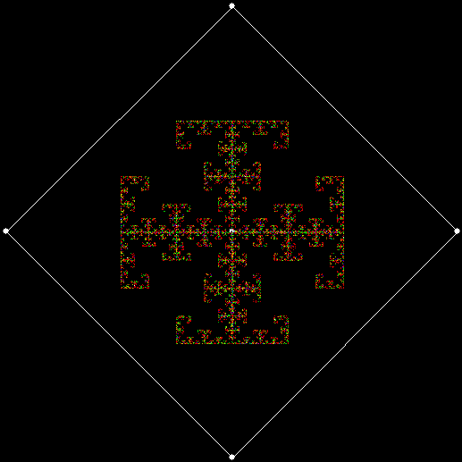

v4_ban12_sw2

v = 4, ban = prox(1), prox(2), sw = 2*

*The second of those fractals is identical to v = 4, ban(prox(2), prox(3)) with a complete bubble-sort.


Here is ban(prox(1), prox(5)) with a complete bubble-sort:
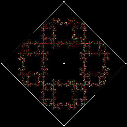
4c_ban15

v = 4, ban = prox(1), prox(5)


Now try ban(prox(1), prox(5)) with an incomplete bubble-sort:

v4_ban15_sw1

v = 4, ban = prox(1), prox(5), sw = 1


v4_ban15_sw2

v = 4, ban = prox(1), prox(5), sw = 2


When sweep = 3, the fractal I had seen before appears:

v4_ban15_sw3

v = 4, ban = prox(1), prox(5), sw = 3


v4_ban15_sw3_anim

v = 4, ban = prox(1), prox(5), sw = 3 (animated)


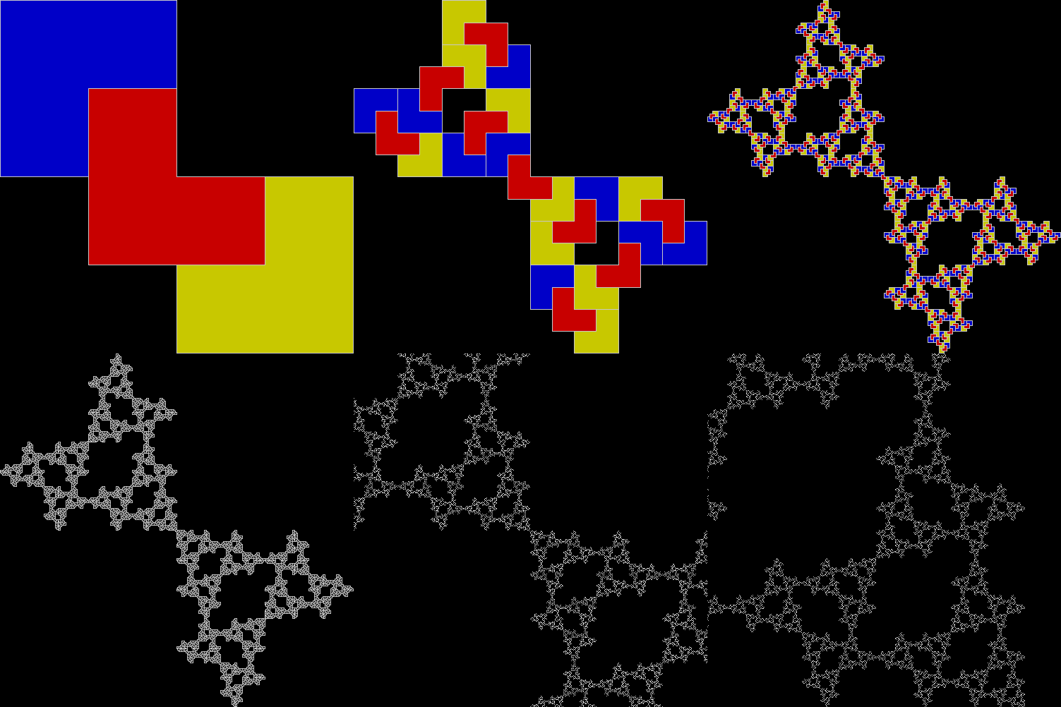
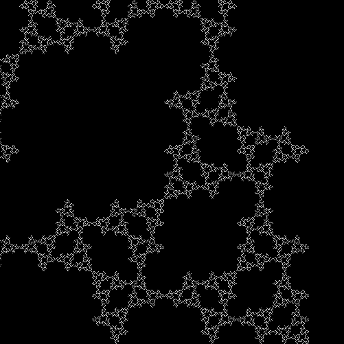
Where had I seen it before? While investigating this rep-tile (a shape that can be tiled with smaller versions of itself):
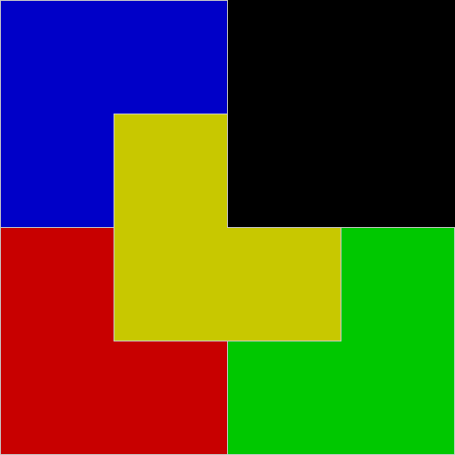
L-reptile

L-triomino rep-tile


L-reptile_anim

L-triomino rep-tile (animated)


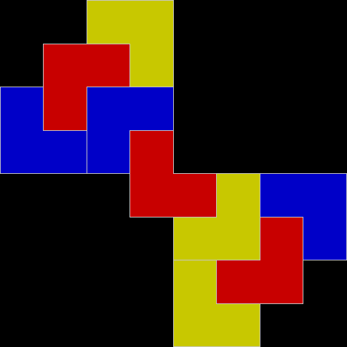
The rep-tile is technically called an L-triomino, because it looks like a capital L and is one of the two distinct shapes you can create by joining three squares at the edges. You can create fractals from an L-triomino by dividing it into four copies, discarding one of the copies, then repeating the divide-and-discard at smaller and smaller scales:

L-reptile_1

L-triomino fractal stage #1


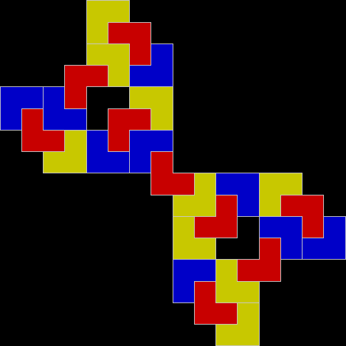
L-reptile_2

L-triomino fractal stage #2


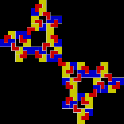
L-reptile_3

L-triomino fractal stage #3


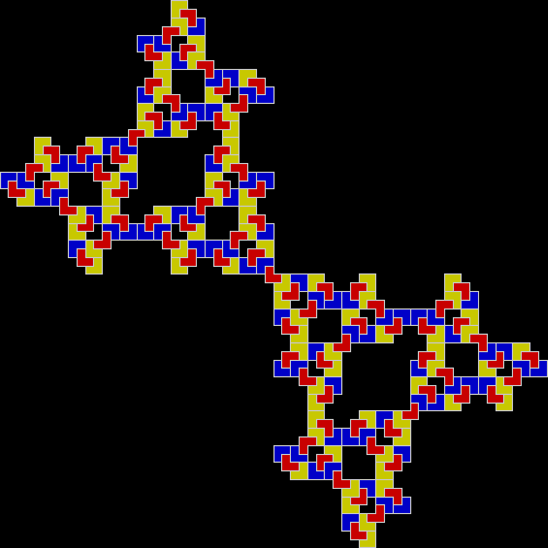
L-reptile_4

L-triomino fractal stage #4


L-reptile_5

L-triomino fractal stage #5


L-reptile_fractal_anim

L-triomino fractal (animated)

L-reptile_fractal_static

L-triomino fractal (close-up)

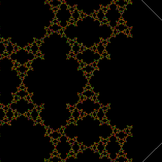
And here’s part of the ban(prox(1), prox(5)) fractal for comparison:
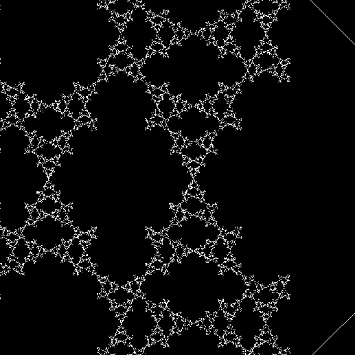
v4_ban15_sw3_mono


v4_ban15_sw3_col

So you can get to the same fractal (or versions of it), by two apparently different routes: random movement of a point inside a square or repeatedly dividing-and-discarding the sub-copies of an L-triomino. That’s serendipity!


Previously pre-posted:

Get Your Prox Off

Radical Sheet

If you take a sheet of standard-sized paper and fold it in half from top to bottom, the folded sheet has the same proportions as the original, namely √2 : 1. In other words, if x = √2 / 2, then 1 / x = √2:
√2 = 1.414213562373…, √2 / 2 = 0.707106781186…, 1 / 0.707106781186… = 1.414213562373…

So you could say that paper has radical sheet (the square or other root of a number is also called its radix and √ is known as the radical sign). When a rectangle has the proportions √2 : 1, it can be tiled with an infinite number of copies of itself, the first copy having ½ the area of the original, the second ¼, the third ⅛, and so on. The radical sheet below is tiled with ten diminishing copies of itself, the final two having the same area:

papersizes

papersizes_static

You can also tile a radical sheet with six copies of itself, two copies having ¼ the area of the original and four having ⅛:

paper_6div_static

paper_6div

This tiling is when you might say the radical turns crucial, because you can create a fractal cross from it by repeatedly dividing and discarding. Suppose you divide a radical sheet into six copies as above, then discard two of the ⅛-sized rectangles, like this:

paper_cross_1

Stage 1


Then repeat with the smaller rectangles:

paper_cross_2

Stage 2


paper_cross_3

Stage 3


paper_cross_4

Stage 4


paper_cross_5

Stage 5


paper_cross

Animated version

paper_cross_static

Fractile cross

The cross is slanted, but it’s easy to rotate the original rectangle and produce an upright cross:

paper_cross_upright

paper_cross_upright_static

Performativizing the Polygonic

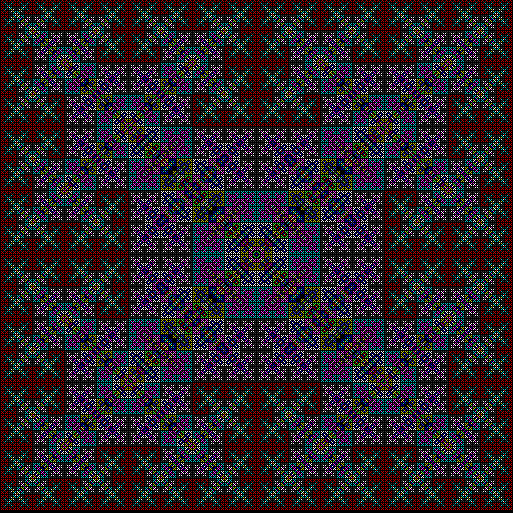
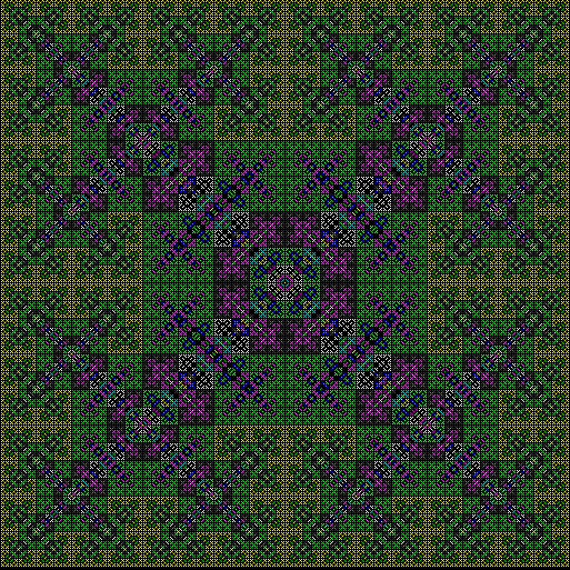
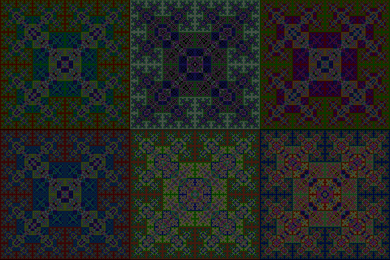
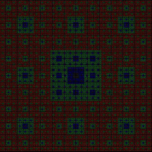
Maths is a mountain: you can start climbing in different places and reach the same destination. There are many ways of proving the irrationality of √2 or the infinitude of the primes, for example. But you can also arrive at the same destination by accident. I’ve found that when I use different methods of creating fractals. The same fractals appear, because apparently different algorithms are actually the same underneath.

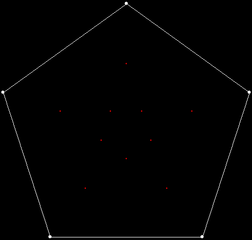
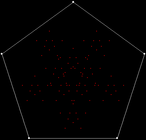
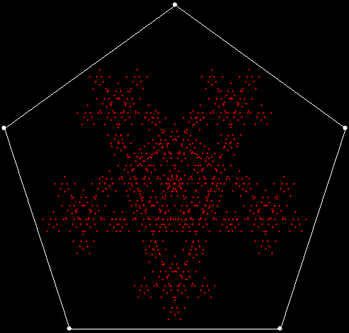
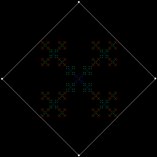
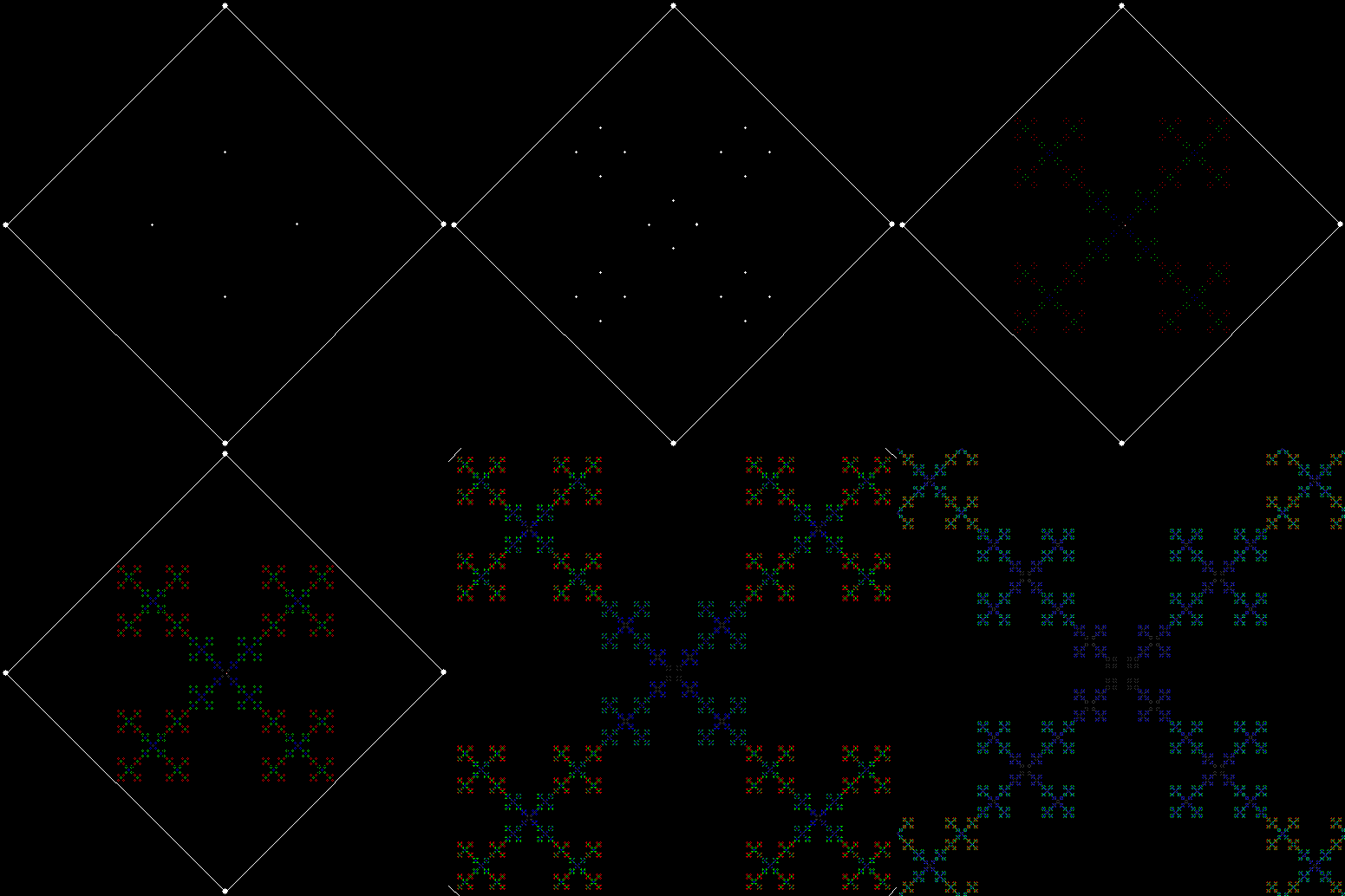
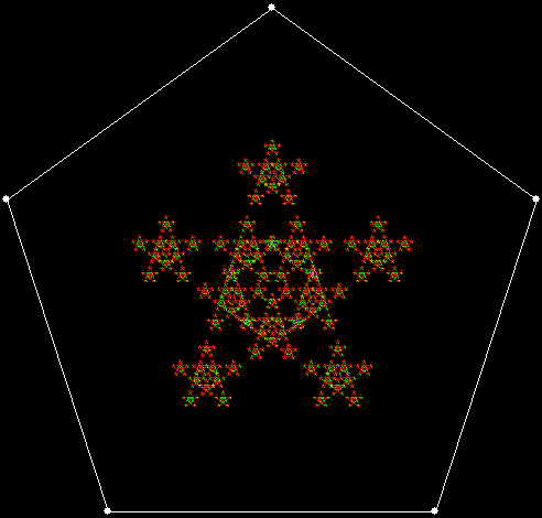
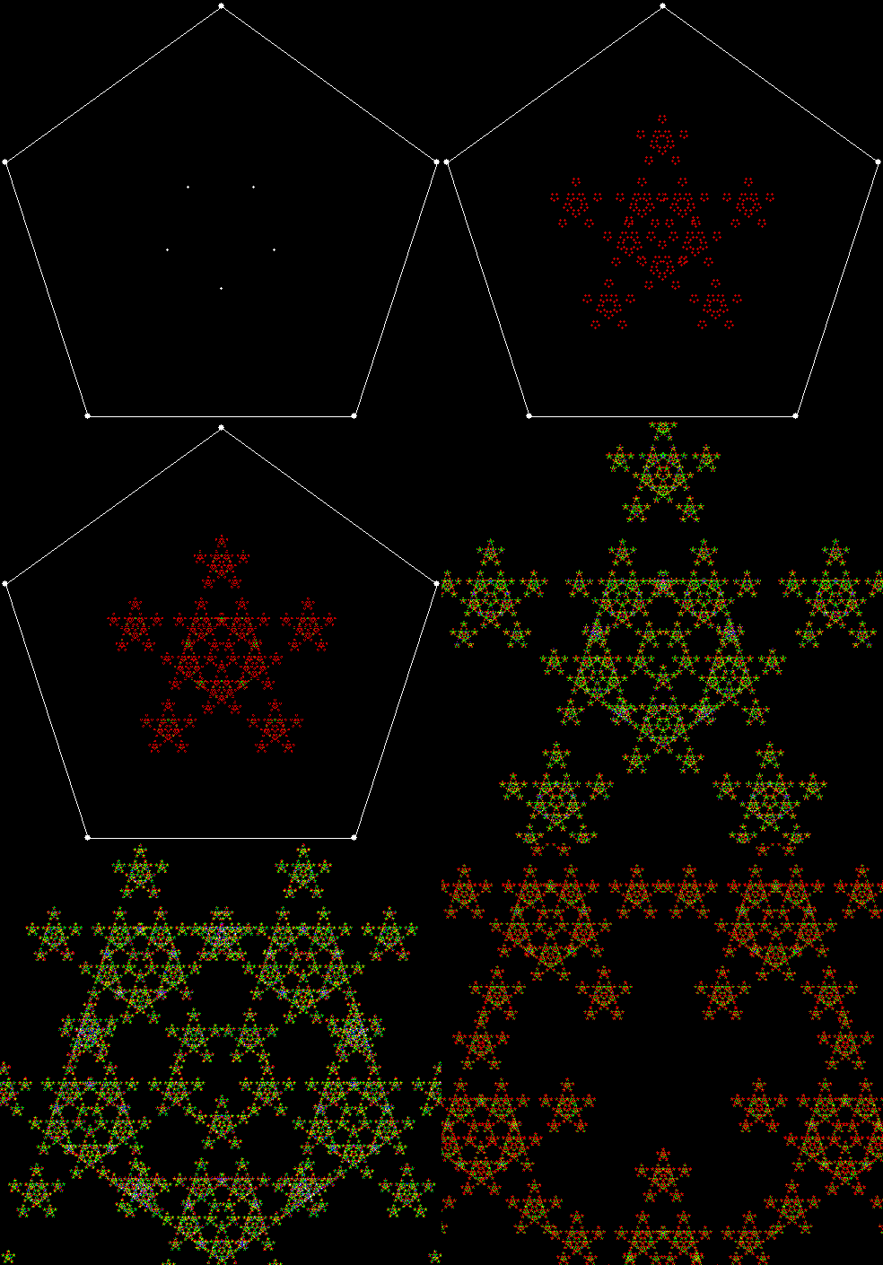
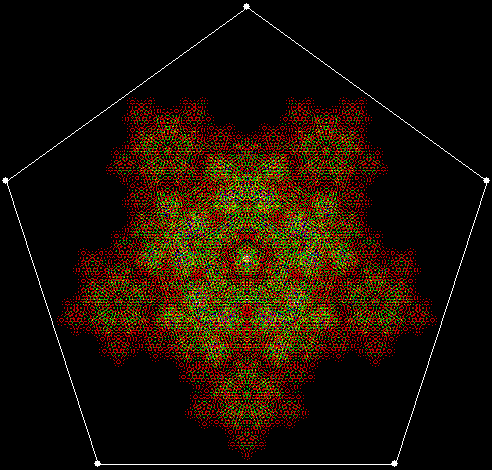
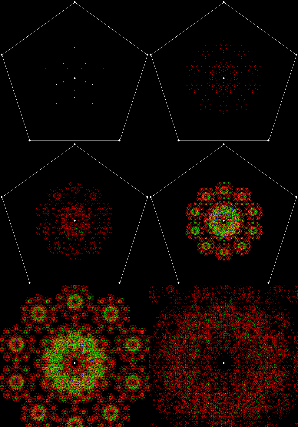
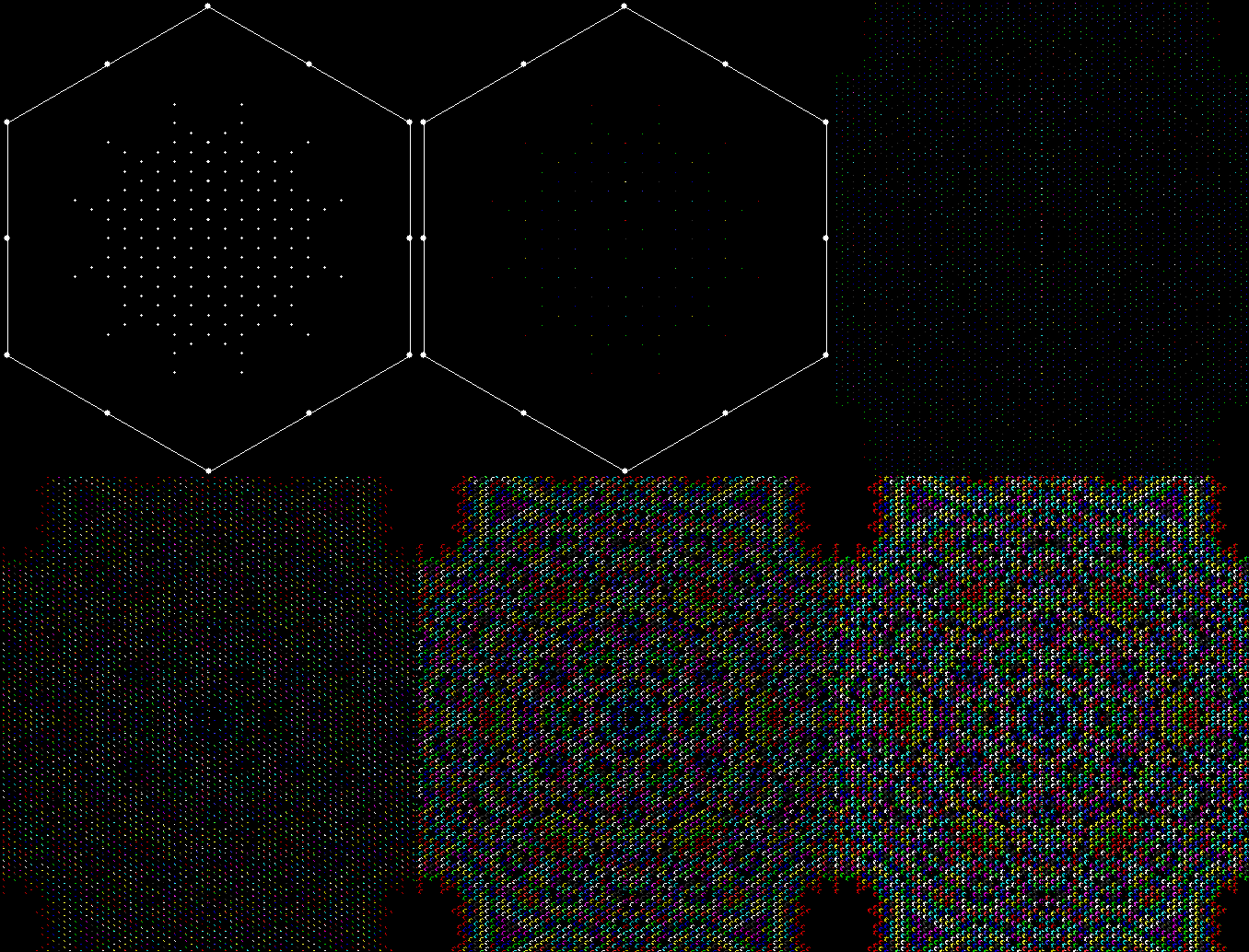
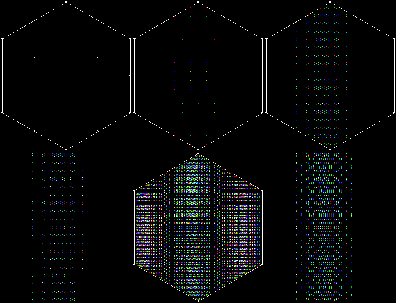
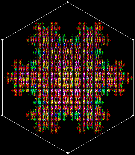
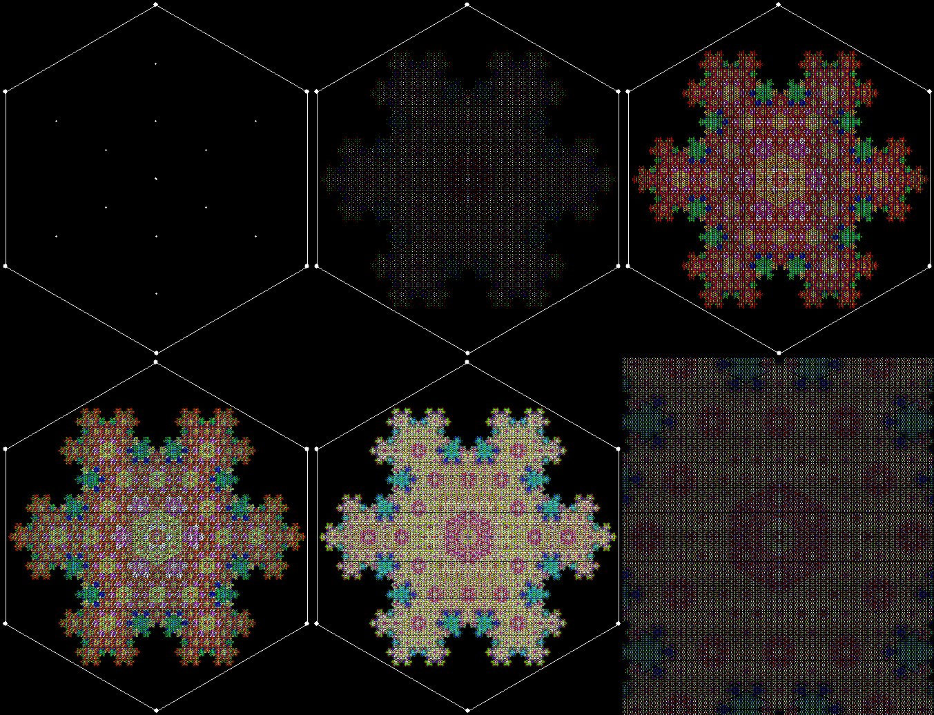
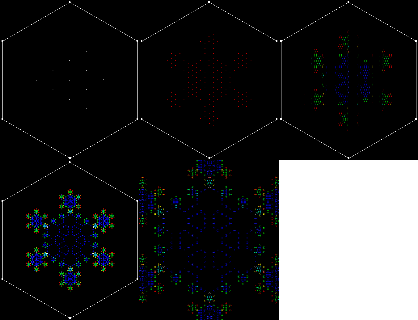
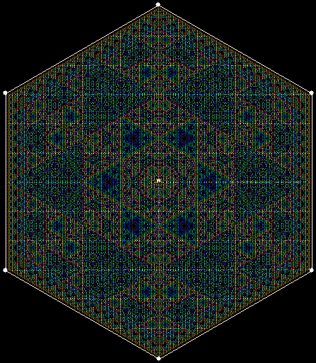
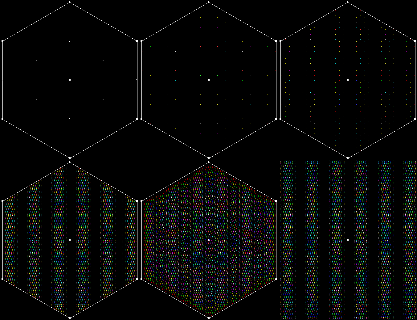
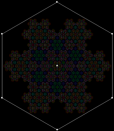
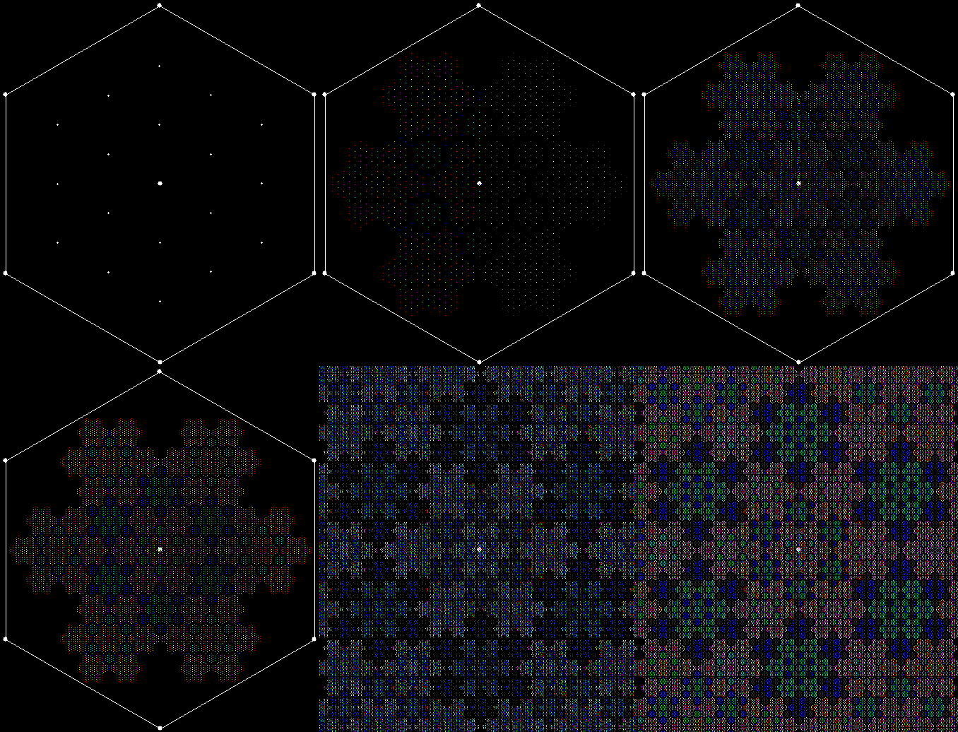
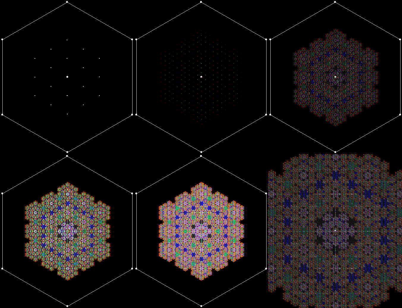
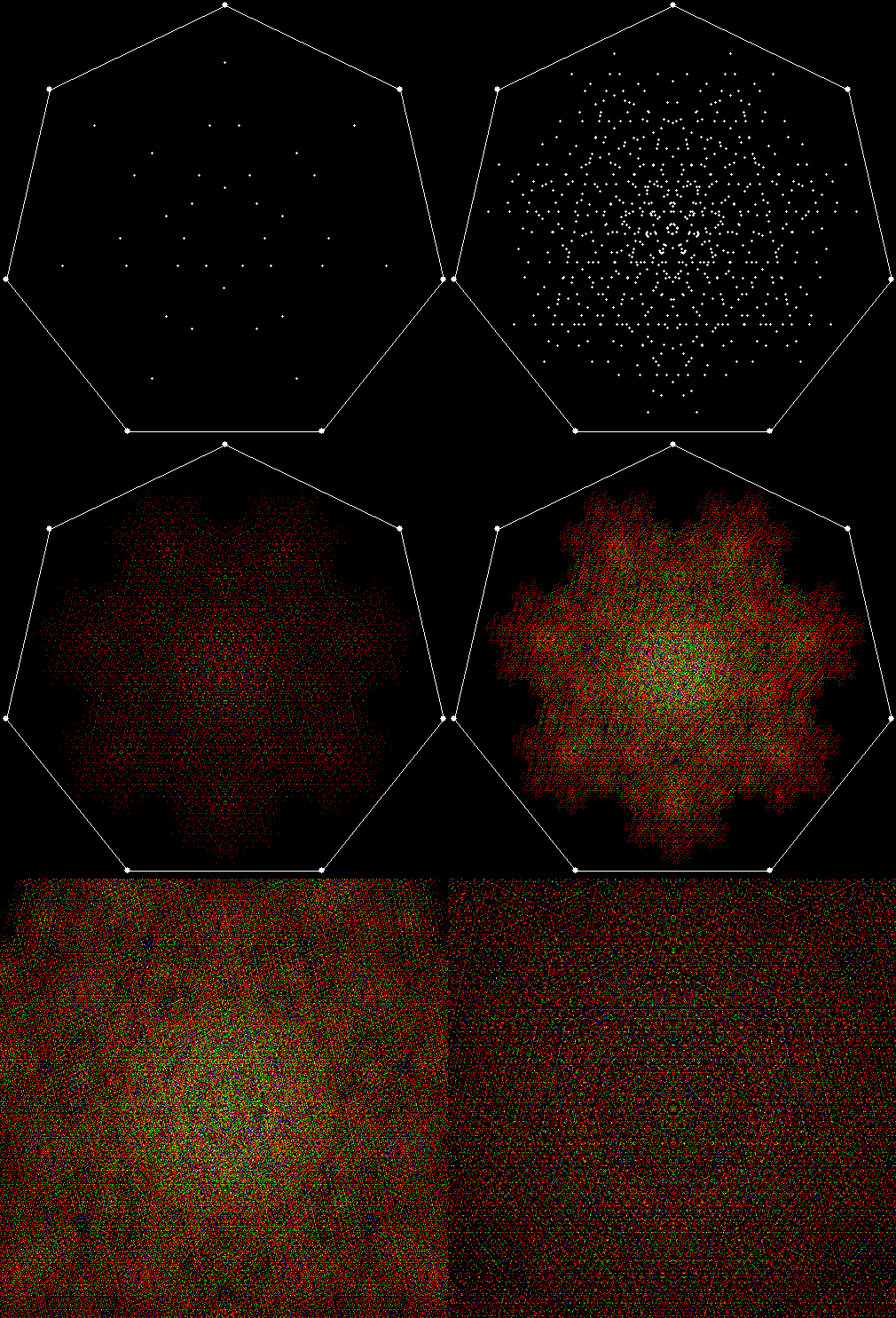
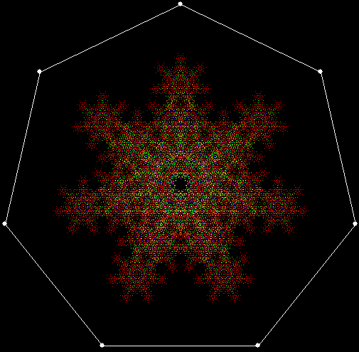
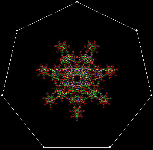
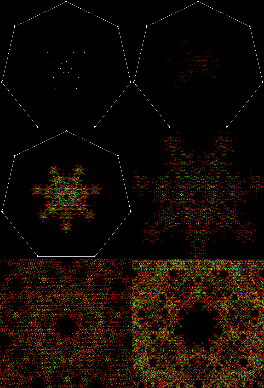
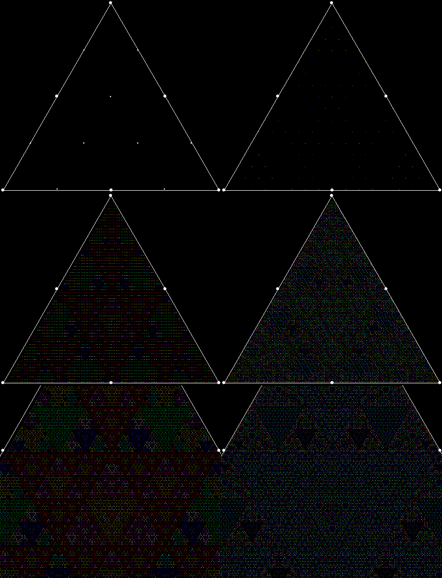
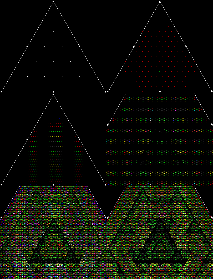
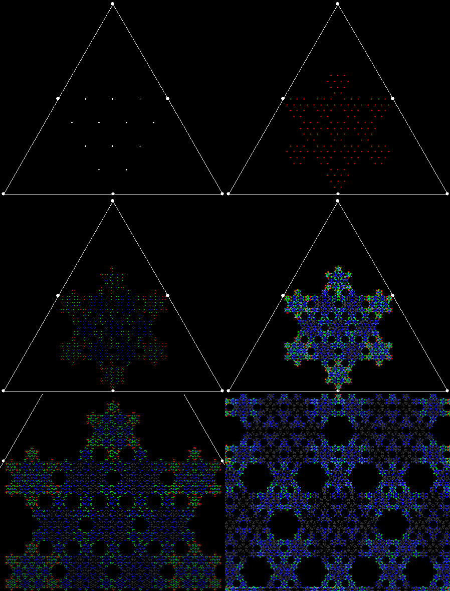
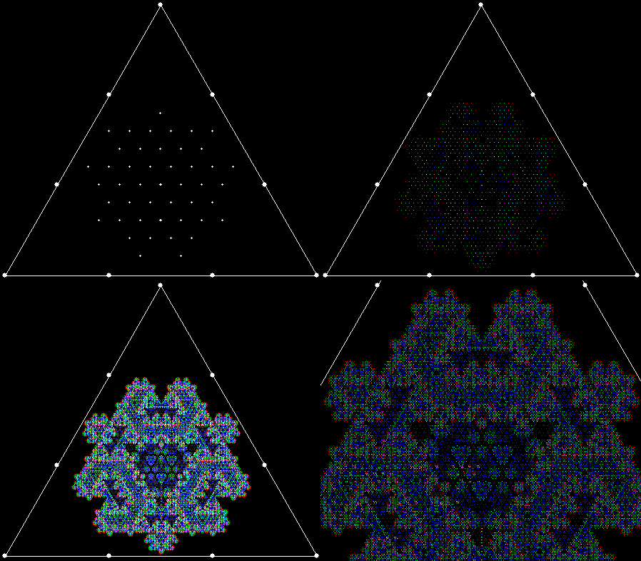
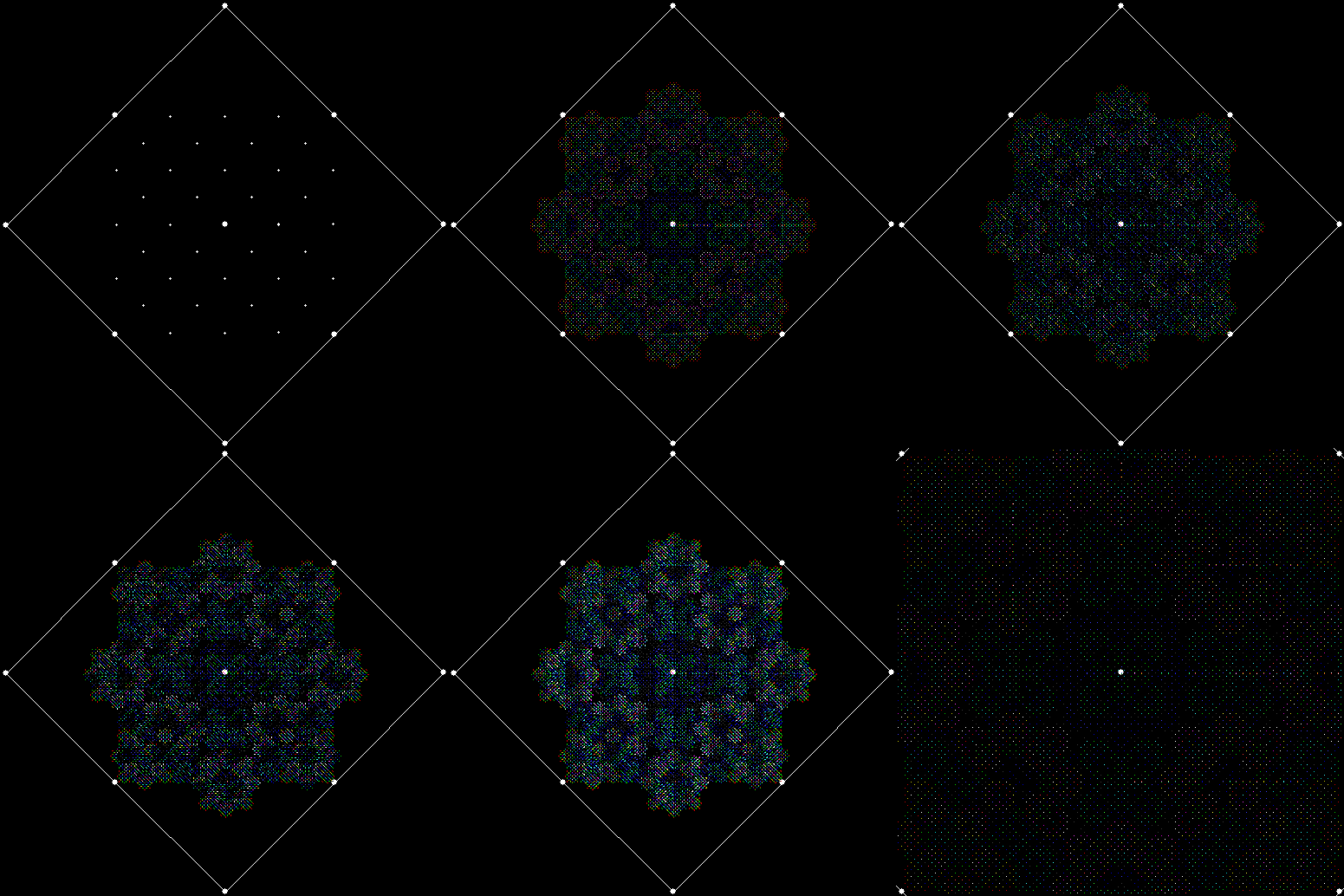
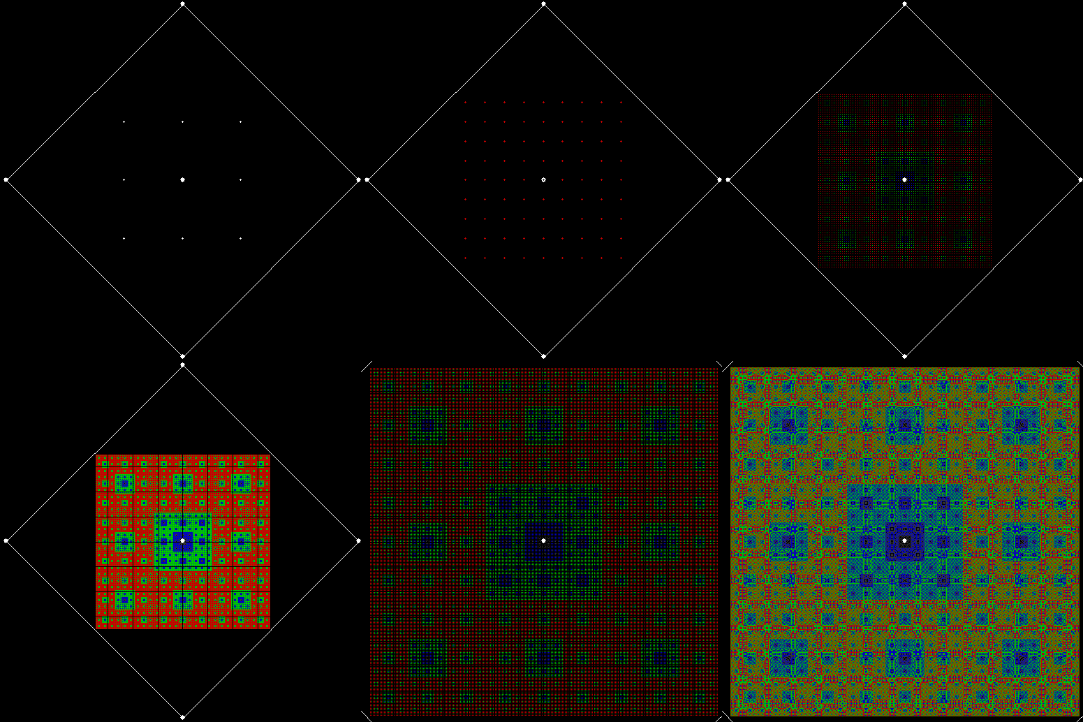
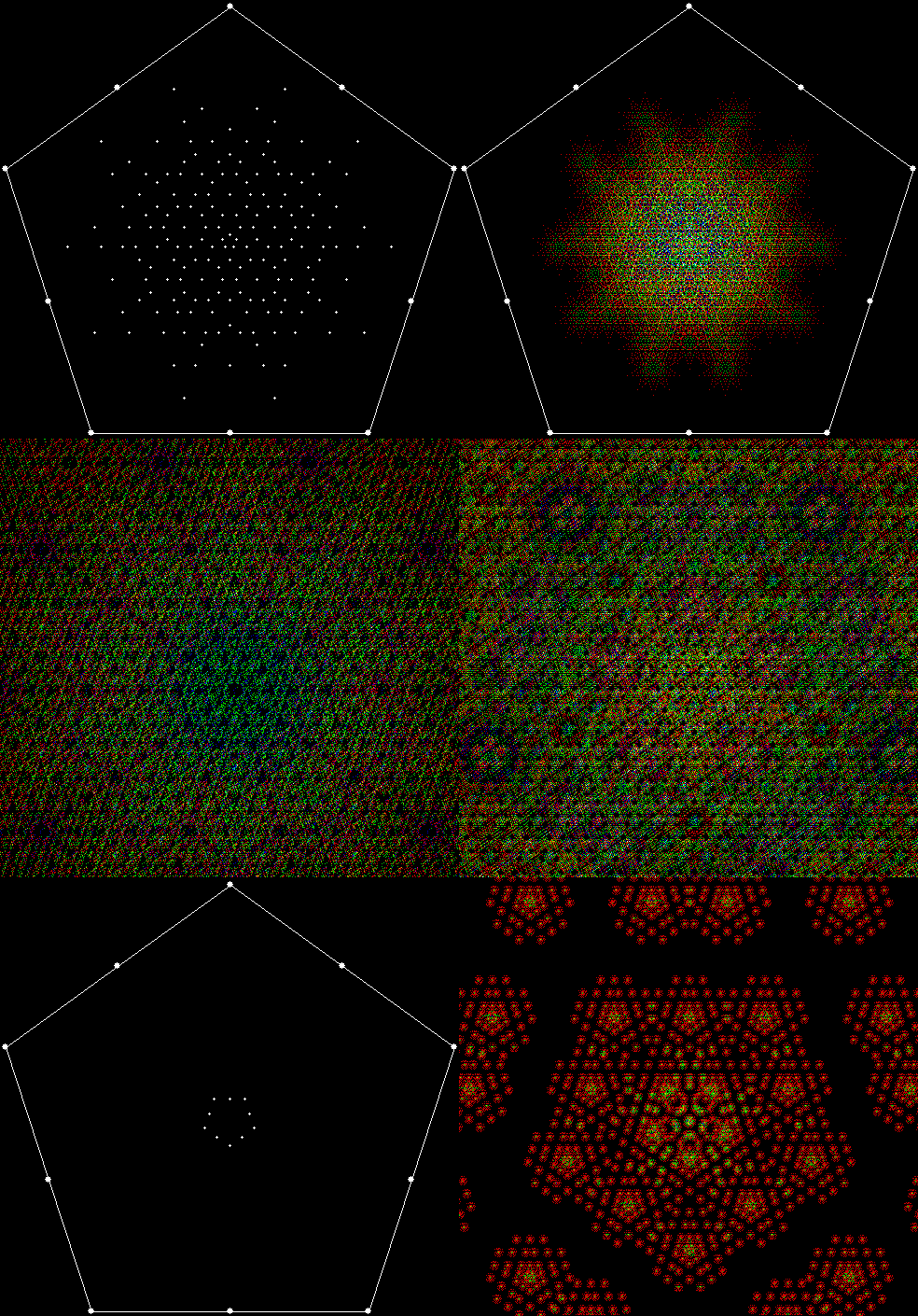
But different methods can create unique fractals too. I’ve found some new ones by using what might be called point-to-point recursion. For example, there are ten ways to select three vertices from the five vertices of a pentagon: (1, 2, 3), (1, 2, 4), (1, 2, 5), (1, 3, 4), (1, 3, 5), (1, 4, 5), (2, 3, 4), (2, 3, 5), (2, 4, 5), (3, 4, 5). Find the midpoint of the first three-point set, (1, 2, 3). Then select two vertices to go with this midpoint, creating a new three-point set, and find the midpoint again. And so on. The process looks like this, with the midpoints shown for all the three-point sets found at each stage:

v5_p3_stage1

vertices = 5, choose sets of 3 points, find mid-point of each

v5_p3_stage2

v5_p3_stage3


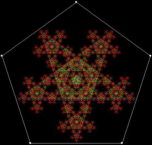
At stage 5, the fractal looks like this:

v5_p3_static

v = 5, p = 3


Note that when pixels are used again, the colour changes. That’s another interesting thing about maths: limits can sometimes produce deeper results. If these fractals were drawn at very high resolution, pixels would only be used once and the colour would never change. As it is, low resolution means that pixels are used again and again. But some are used more than others, which is why interesting colour effects appear.

If the formation of the fractal is animated, it looks like this (with close-ups of even deeper stages):
v5_p3


Here are some more examples:

v4c_p2_static

v = 4 + central point, p = 2 (cf. Fingering the Frigit)

v4c_p2

v = 4c, p = 2 (animated)


v4_p3_static

v = 4, p = 3

v4_p3


v5_p4_static

v = 5, p = 4

v5_p4


v5c_p3_static

v = 5 + central point, p = 3

v5c_p3


v5c_p4

v = 5c, p = 4


v5c_p5

v = 5c, p = 5


v6_1_p6

v = 6 + 1 point between each pair of vertices, p = 6


v6_p2

v = 6, p = 2


v6_p3_static

v = 6, p = 3

v6_p3


v6_p4

v = 6, p = 4


v6c_p2_static

v = 6c, p = 2 (cf. Fingering the Frigit)

v6c_p2


v6c_p3_static

v = 6c, p = 3

v6c_p3


v6c_p4

v = 6c, p = 4


v7_p3

v = 7, p = 3


v7_p4_static

v = 7, p = 4

v7_p4


v7_p5_static

v = ,7 p = 5

v7_p5


v7_p4

v = 7c, p = 4


v3_1_p2

v = 3+1, p = 2


v3_1_p3

v = 3+1, p = 3


v3_1_p4

v = 3+1, p = 4


v3_2_p5

v = 3+2, p = 5


v3c_1_p2

v = 3c+1, p = 2


v3c_1_p4

v = 3c+1, p = 4


v3c_p2

v = 3c, p = 2


v3c_p3

v = 3c, p = 3


v4_1_p3

v = 4+1, p = 3


v4_1_p4

v = 4+1, p = 4


v4_1_p5

v = 4+1, p = 6


v4_1_p6

v = 4+1, p = 2


v4c_1_p4

v = 4c+1, p = 4


v4c_p3_static

v = 4c, p = 3

v4c_p3


v5_1_p4_va

v = 5+1, p = 4 (and more)


v5_p2

v = 5, p = 2