Polymorphous Pursuit

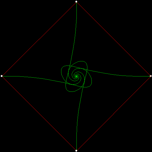
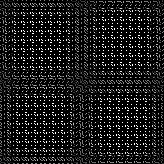
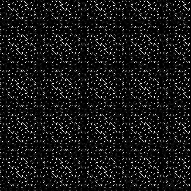
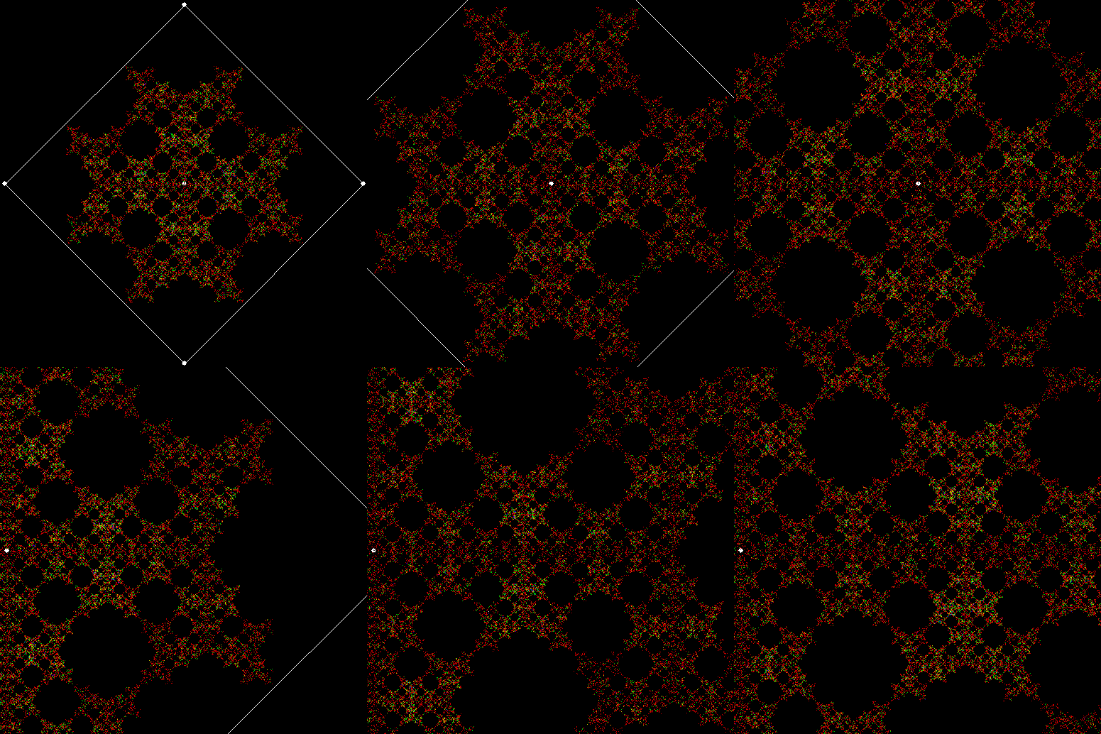
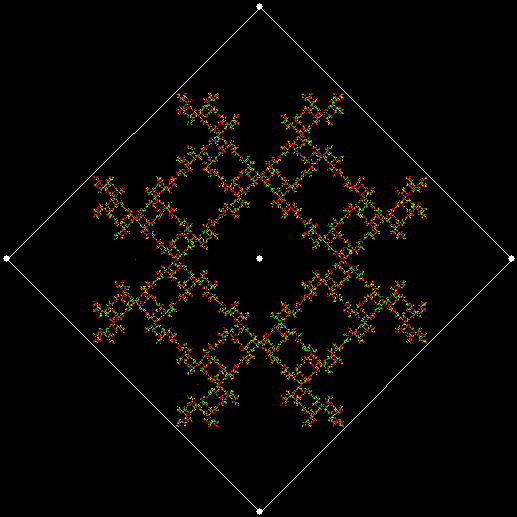
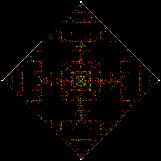
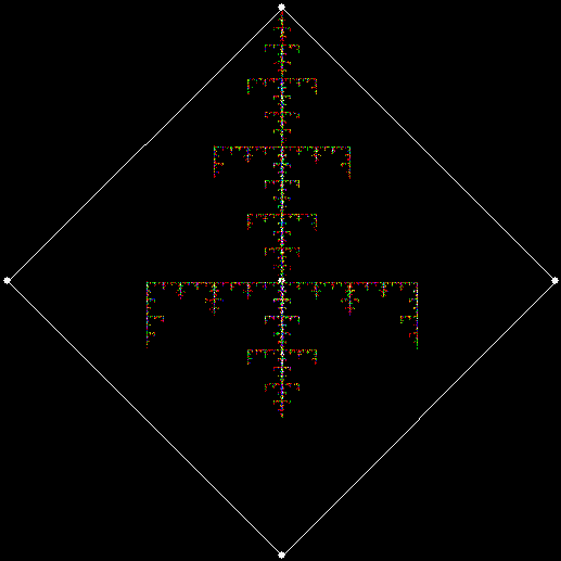
Suppose four mice are standing on the corners of a large square. Each mouse begins running at the same speed towards the mouse one place away, reckoning clockwise. The mice will meet at the centre of the square and the path taken by each mouse will be what is known as a pursuit curve:
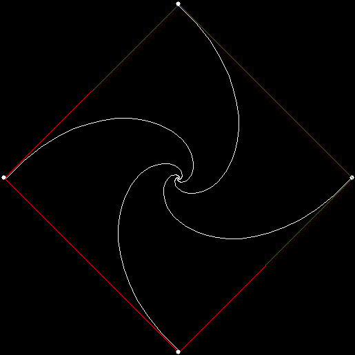
v4_mi1

vertices = 4, mouse-increment = 1


v4_mi1_animated

v = 4, mi = 1 (animated)


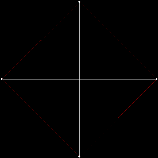
As I showed in “Persecution Complex”, it’s easy to find variants on the basic pursuit curve. If mi = 2, i.e. each mouse runs towards the mouse two places away, the mice will run in straight lines direct to the centre of the square:
v4_mi2

v = 4, mi = 2


v4_mi2_animated

v = 4, mi = 2 (animated)


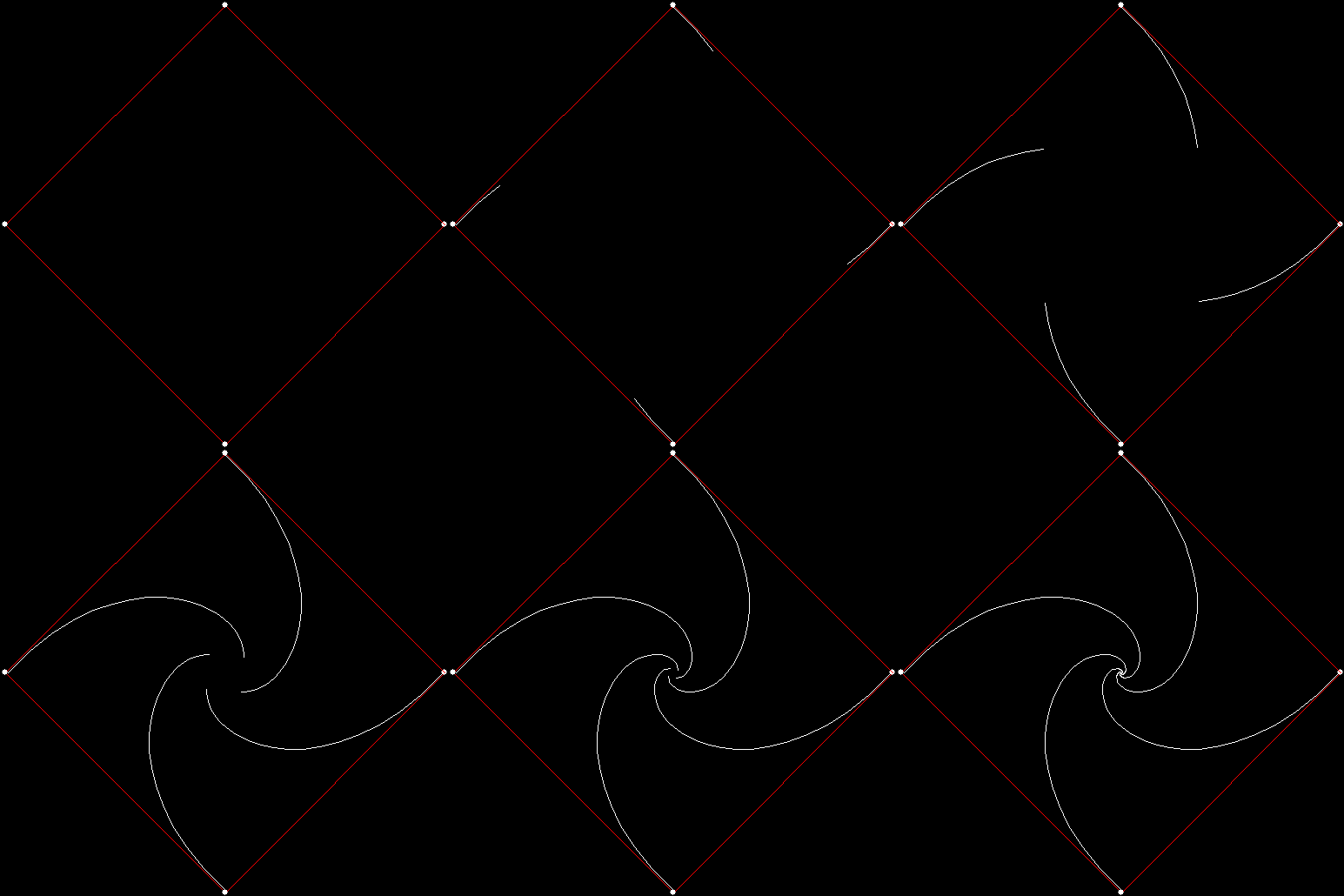
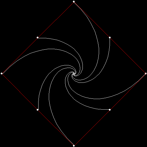
That variant is trivial, but suppose there are eight mice, four starting on the corners of the square and four starting on the midpoints of the sides. Mice starting on the corners will run different pursuit curves to those starting on the midpoints, because the corners are further from the centre than the midpoints are:
v4_si1_mi1

v = 4, si = 1, mi = 1


v4_si1_mi1_extra


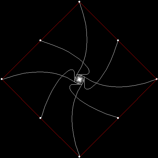
If mi = 3, the pursuit curves look like this:
v4_si1_mi3

v = 4, si = 1, mi = 3


v4_si1_mi3_animated

v = 4, si = 1, mi = 3 (animated)


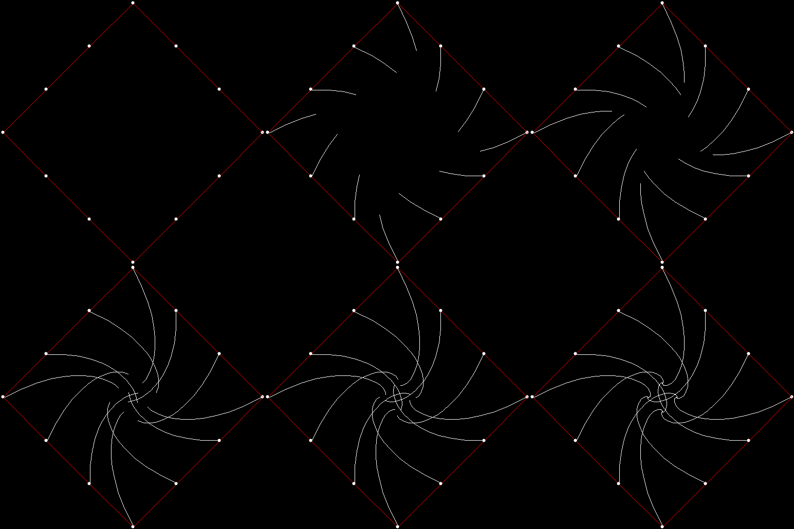
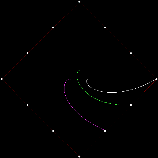
Suppose there are twelve mice, four on each corner and two more on each side. If each mouse runs towards the mouse four places away, then the pursuit curves don’t all meet in the centre of the square. Instead, they meet in groups of three at four points equidistant from the centre, like this:

v4_si2_mi4

v4_si2_mi4_curves

v = 4, si = 2, mi = 4


v4_si2_mi4_animated

v = 4, si = 2, mi = 4 (animated)


v4_si4_mi4_animated

v = 4, si = 4, mi = 4 (animated)


v4_si4_mi4_large

v = 4, si = 4, mi = 4 (zoom)


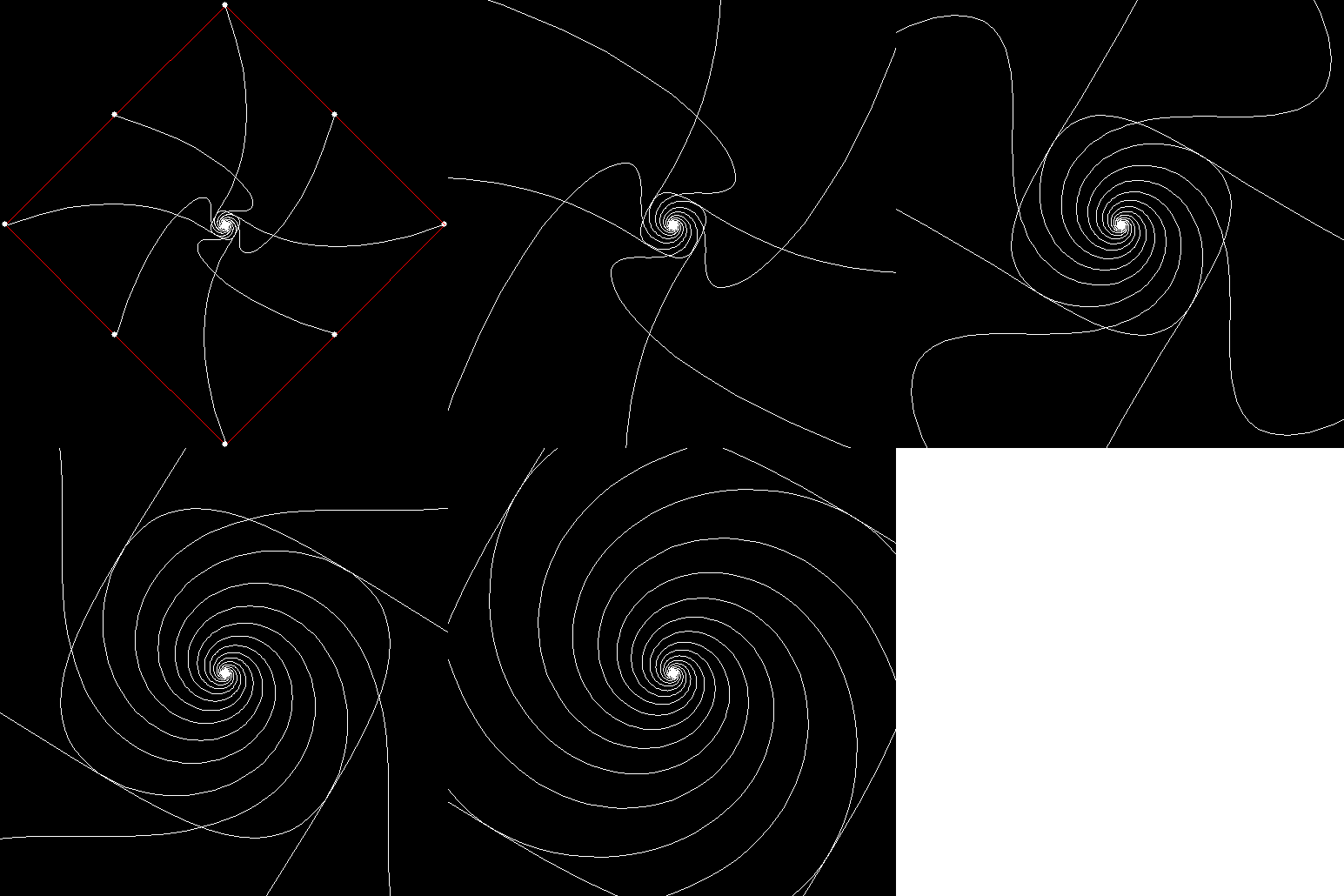
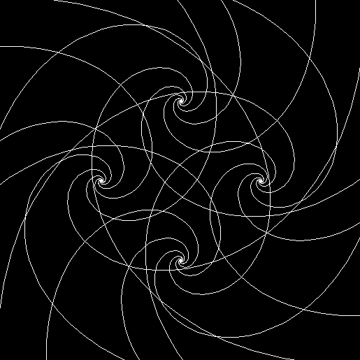
Now suppose each mouse become sophisticated and runs toward the combined positions of two other mice, one two places away, the other three places away, like this:

v4_si1_mi2_3

v = 4, si = 1, mi = (2, 3)


v4_si1_mi2_3_animated

v = 4, si = 1, mi = (2, 3) (animated)


These polypursuits, as they could be called, can have complicated central regions:
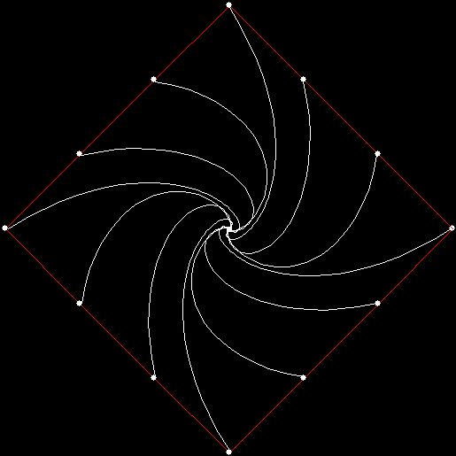
v4_si2_mi1_4

v = 4, si = 2, mi = (1, 4)


v4_si2_mi1_4_animated

v = 4, si = 2, mi = (1, 4) (animated)
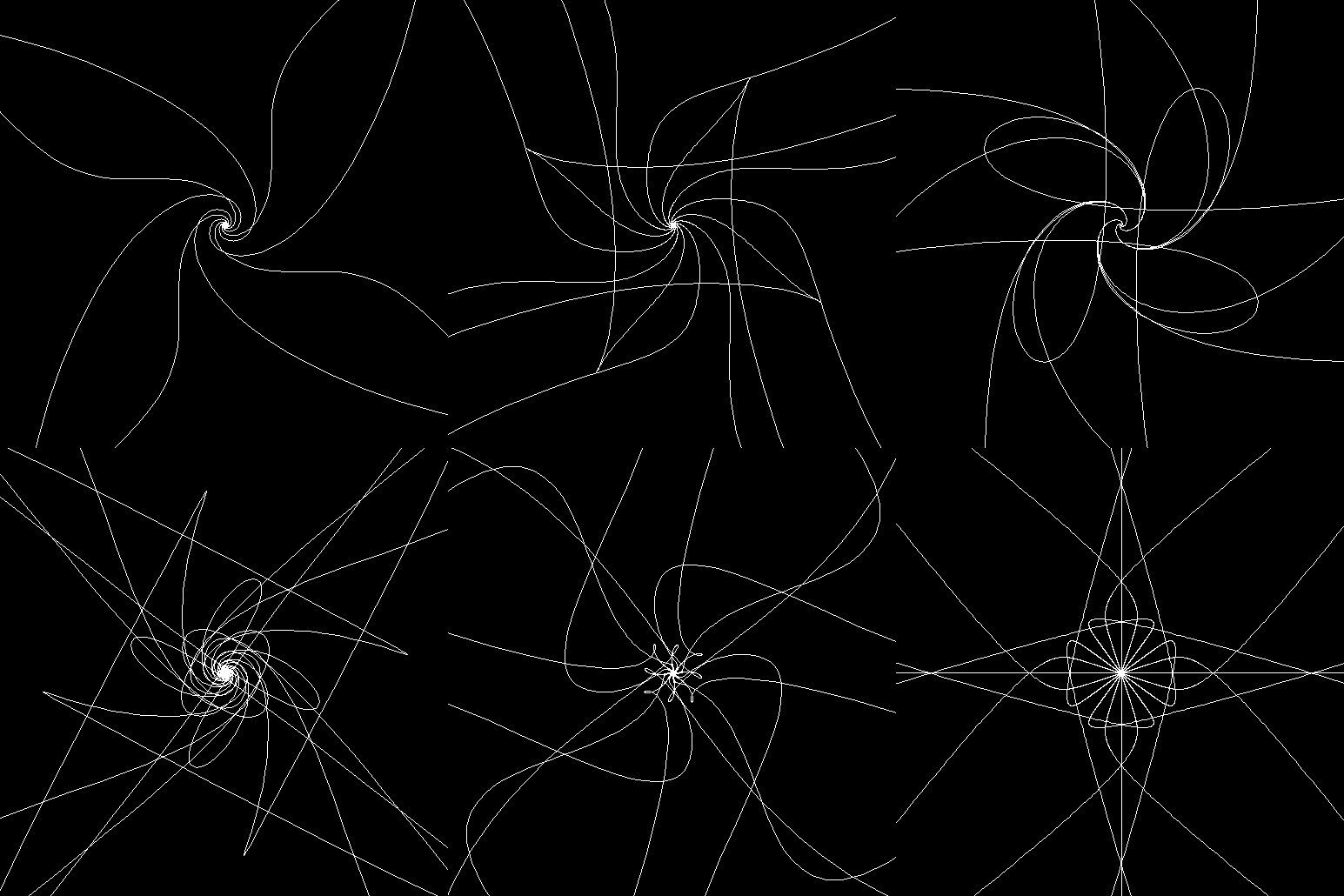

v4_si_va_mi_va

v = 4, si = various, mi = various


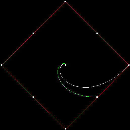
And what if you have two teams of mice, running towards one or more mice on the other team? For example, suppose two mice, one from each team, start on each corner of a square. Each mouse on team 1 runs towards the mouse on team 2 that is one place away, while each mouse on team 2 runs towards the mouse on team 1 that is two places away. If the pursuits curves of team 1 are represented in white and the pursuit curves of team 2 in green, the curves look like this:
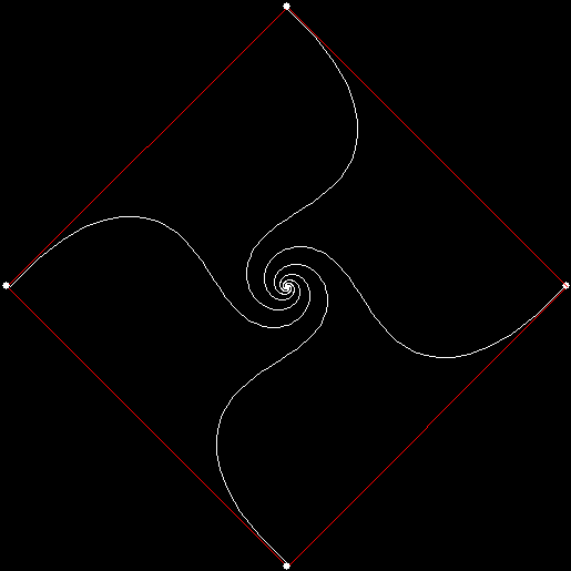
2v4_mi1_mi2

v = 4 * 2, vmi = 1, vmi = 2


2v4_mi1_mi2_green

v = 4 * 2, vmi = 1, vmi = 2


2v4_mi1_mi2_animated

v = 4 * 2, vmi = 1, vmi = 2 (animated)


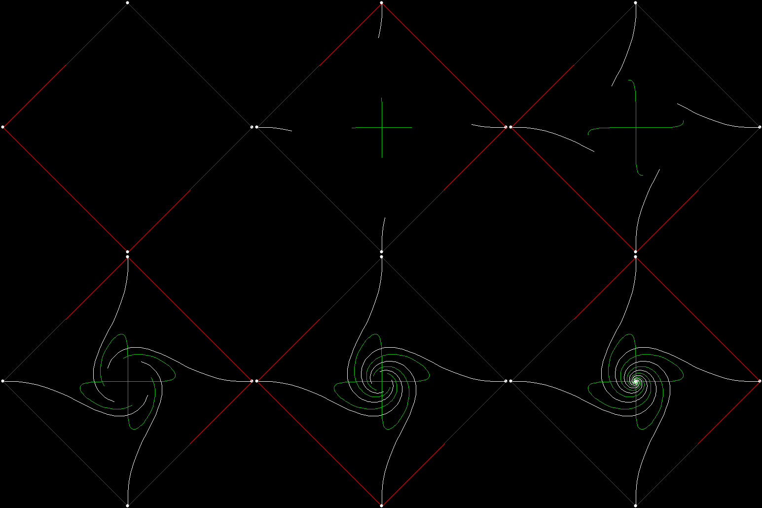
Now suppose the four mice of team 1 start on the corners while the mice of team 2 start at the centre of the square.
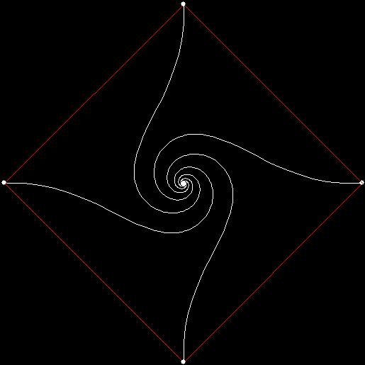
v4_c4_vmi1_cmi2_white

v = 4, centre = 4, vmi = 1, cmi = 2 (white team)


v4_c4_vmi1_cmi2_green

v = 4, centre = 4, vmi = 1, cmi = 2 (green team)


v4_c4_vmi1_cmi2_both

v = 4, centre = 4, vmi = 1, cmi = 2 (both teams)

v4_c4_vmi1_cmi2_animated

v = 4, centre = 4, vmi = 1, cmi = 2 (animated)


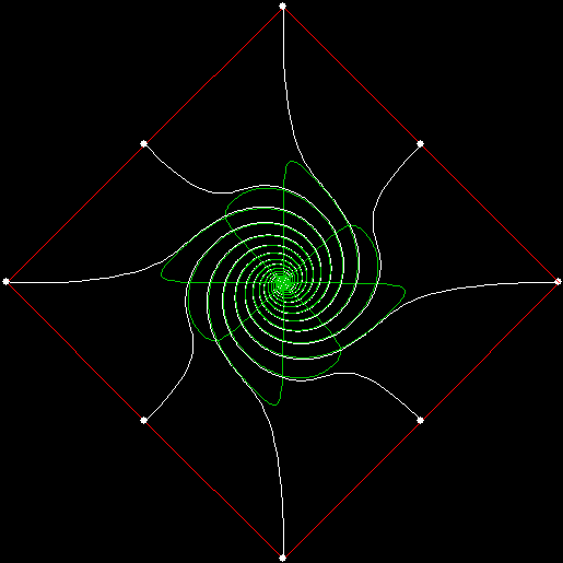
Here are more variants on pursuit curves formed by two teams of mice, one starting on the corners, one at the centre:
v4_c4_vmi0_1_cmi0

v = 4, centre = 4, vmi = (0, 1), cmi = 0


v4_c4_vmi0_2_cmi0

v = 4, centre = 4, vmi = (0, 2), cmi = 0


v4_c4_vmi0_3_cmi0

v = 4, centre = 4, vmi = (0, 3), cmi = 0


2v4_mi1_mi2_both

White Rites

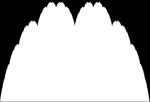
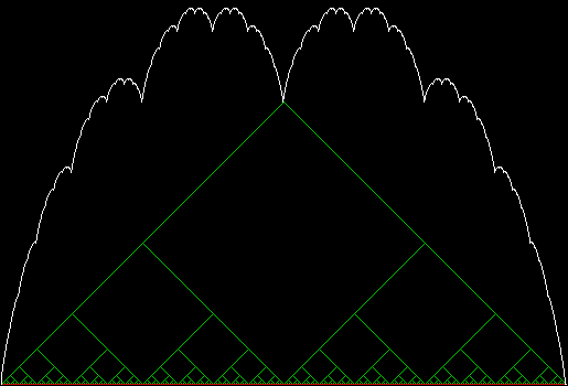
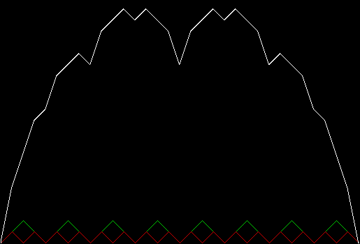
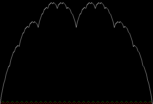
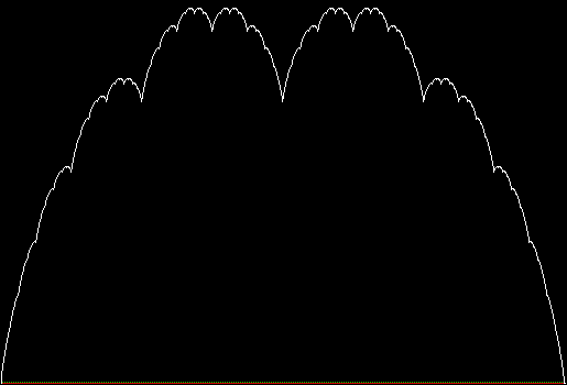
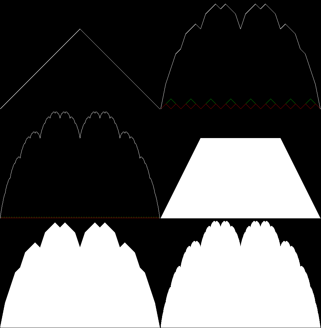
The blancmange curve is an interesting fractal formed by summing a series of zigzags. It
takes its name from its resemblance to the milk-pudding known as a blancmange
(blanc-manger in French, meaning “white eating”):

blanc_solid

Blancmange curve


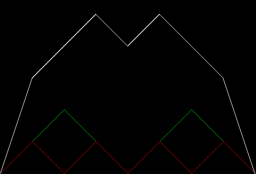
In successive zigzags, the number of zags doubles as their height halves, i.e. z(i) = z(i-1) * 2, h(i) = h(i-1) / 2. If all the zigzags are represented at once, the construction looks like this:

blanc_all

Zigzags 1 to 10


blancmange_all

Zigzags 1 to 10 (animated)


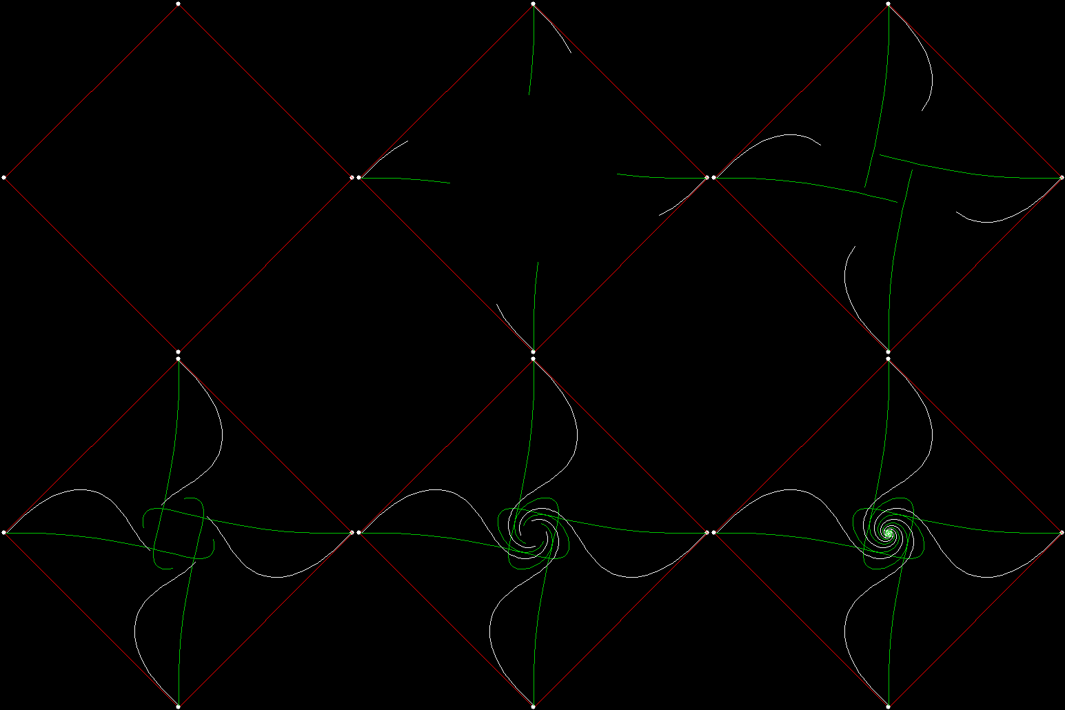
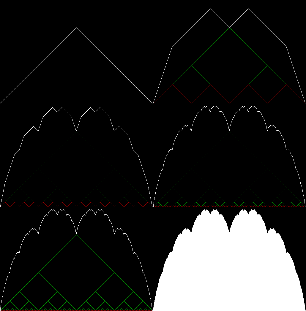
Here is a step-by-step construction, with the total sum of zigzags in white, the present zigzag in red and the previous zigzag in green:

blanc1

Blancmange curve stage 1


blanc2

Stage 2


blanc3

Stage 3


blanc4

Stage 4


blanc5

Stage 5


blanc6

Stage 6


blanc7

Stage 7


blanc8

Stage 8


blanc9

Stage 9


blanc10

Stage 10


blancmange

Blancmange curve (animated)


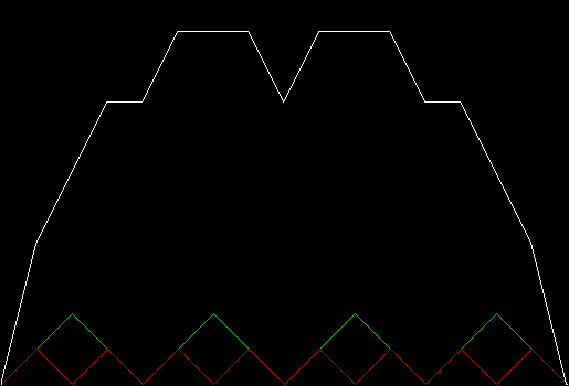
It’s easy to think of variants on the standard blancmange curve. Suppose the number of zags triples as their height is divided by three, i.e. z(i) = z(i-1) * 3, h(i) = h(i-1) / 3:

blanc_x3_solid

Blancmange curve for z(i) = z(i-1) * 3, h(i) = h(i-1) / 3


Continue reading “White Rites”…

Bash the Pash

An heretical Guardianista keyly critiquizes a core component of Guardianese:

I recently considered nominating for a board position on a professional association to which I belong, so I had a look at the biographical statements of the incumbents. One claimed to be “passionate about helping individuals, businesses, and communities thrive”, another declared “a particular passion for thought leadership and executive profiling”, and another revealed “a passion for social inclusion”. Yet another claimed “a passion about creating valuable career development opportunities for the profession”. The best was the one that stated, without irony, “a passion for working on meaningful projects”.

In days gone by, job applicants listed hobbies. These days, it appears candidates are expected to declare, not merely interests or things they like doing, but things they are allegedly passionate about. — Being enthusiastic is no longer enough. Now we must all be passionate, Paul Begley, The Guardian, 13/vii/2016.


Elsewhere other-engageable:

• Ex-term-in-ate!
• Reds under the Thread
• Titus Graun — Heresy, Homotextuality, Hive-Mind
• Oh My Guardian

Performativizing Papyrocentricity #49

Papyrocentric Performativity Presents:

• Clarke’s Sparks – The Collected Stories, Arthur C. Clarke (Victor Gollancz 2000)

• Deeper and Down – Blind Descent: The Quest to Discover the Deepest Place on Earth, James M. Tabor (Random House 2010)

• Manchester’s Mozzerabilist Messiah – Morrissey: The Pageant of His Bleeding Heart, Gavin Hopps (Continuum Books 2012)


• Or Read a Review at Random: RaRaR

Toxic Turntable #6

Currently listening…

• Anaïd, Magna Est (1969)
• Linnet, Venussong (1977)
• Šrúsma, Ðrioso (1994)
• Milchstraße, Der Schwarze Zwerg (2001)
• Ser, Acanthocalycium (1989)
• Zélote, Lac d’Angoisse (1992)


Previously pre-posted:

Toxic Turntable #1 • #2 • #3 • #4 • #5 •

Get Your Ox Off

Boustrophedon (pronounced “bough-stra-FEE-dun” or “boo-stra-FEE-dun”) is an ancient Greek word literally meaning “as the ox turns (in ploughing)”, that is, moving left-right, right-left, and so on. The word is used of writing that runs down the page in the same way. To see what that means, examine two versions of the first paragraph of Clark Ashton Smith’s story “The Demon of the Flower” (1933). The first is written in the usual way, the second is written boustrophedon:

Not as the plants and flowers of Earth, growing peacefully beneath a simple sun, were the blossoms of the planet Lophai. Coiling and uncoiling in double dawns; tossing tumultuously under vast suns of jade green and balas-ruby orange; swaying and weltering in rich twilights, in aurora-curtained nights, they resembled fields of rooted servants that dance eternally to an other-worldly music.


Not as the plants and flowers of Earth, growing peacefully
.iahpoL tenalp eht fo smossolb eht erew ,nus elpmis a htaeneb
Coiling and uncoiling in double dawns; tossing tumultuously
;egnaro ybur-salab dna neerg edaj fo snus tsav rednu
swaying and weltering in rich twilights, in aurora-curtained
ecnad taht stnavres detoor fo sdleif delbmeser yeht ,sthgin
eternally to an other-worldly music.


Boustrophedon writing was once common and sometimes the left-right lines would also be mirror-reversed, like this:


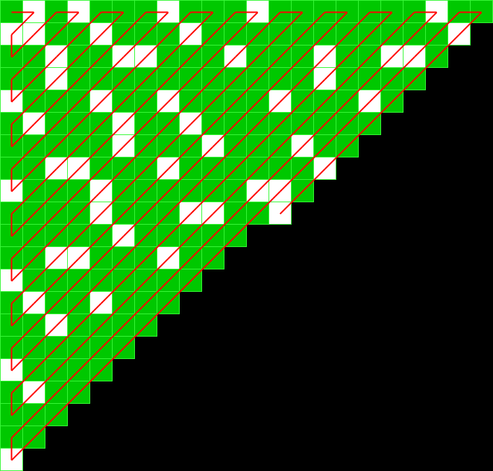
You could also use the term “boustrophedon” to describe the way this table of numbers is filled:

primes_table


The table begins with “1” in the top left-hand corner, then moves right for “2”, then down for “3”, then right-and-up for “4”, “5” and “6”, then right for “7”, then left-and-down for “8”, “9” and “10”, and so on. You could also say that the numbers snake through the table. I’ve marked the primes among them, because I was interested in the patterns made by the primes when the numbers were represented as blocks on a grid, like this:

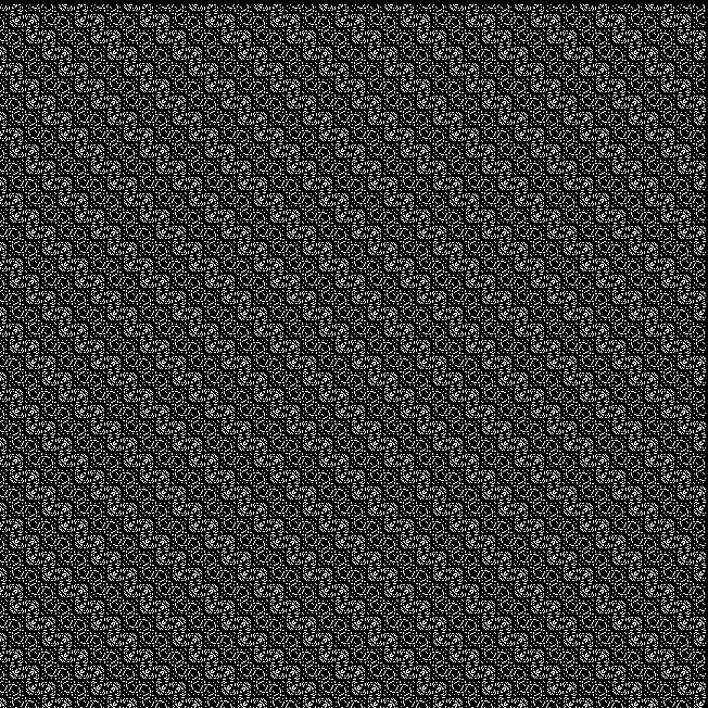
primes_large


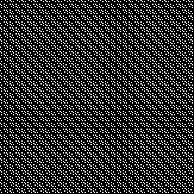
Primes are in solid white (compare the Ulam spiral). Here’s the boustrophedon prime-grid on a finer scale:

primes

(click for full image)


And what about other number-tests? Here are the even numbers marked on the grid (i.e. n mod 2 = 0):

mod2

n mod 2 = 0


And here are some more examples of a modulus test:

mod3

n mod 3 = 0


mod5

n mod 5 = 0
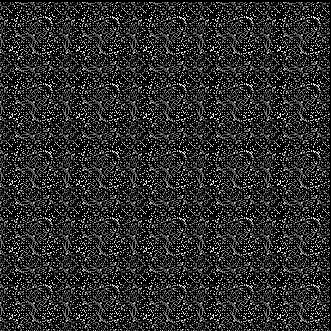

mod9

n mod 9 = 0
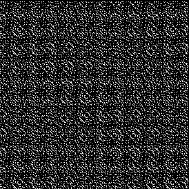

mod15

n mod 15 = 0


mod_various

n mod various = 0 (animated gif)


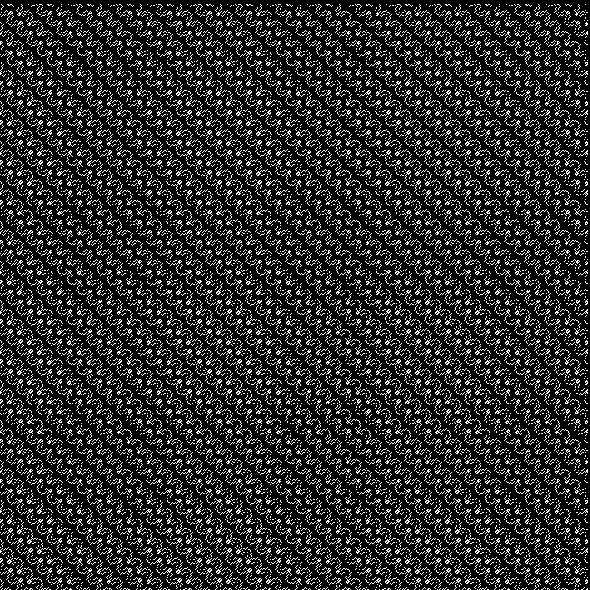
Next I looked at reciprocals (numbers divided into 1) marked on the grid, with the digits of a reciprocal marking the number of blank squares before a square is filled in (if the digit is “0”, the square is filled immediately). For example, in base ten 1/7 = 0.142857142857142857…, where the block “142857” repeats for ever. When represented on the grid, 1/7 has 1 blank square, then a filled square, then 4 blank squares, then a filled square, then 2 blank squares, then a filled square, and so on:

recip7_base10

1/7 in base 10


And here are some more reciprocals (click for full images):

recip9_base2

1/9 in base 2


recip13_base10

1/13 in base 10


recip27_base10

1/27 in base 10


recip41_base10

1/41 in base 10


recip63_base10

1/63 in base 10


recip82_base10

1/82 in base 10


recip101_base10

1/101 in base 10


recip104_base10

1/104 in base 10


recip124_base10

1/124 in base 10


recip143_base10

1/143 in base 10


recip175_base10

1/175 in base 10


recip604_base8

1/604 in base 8


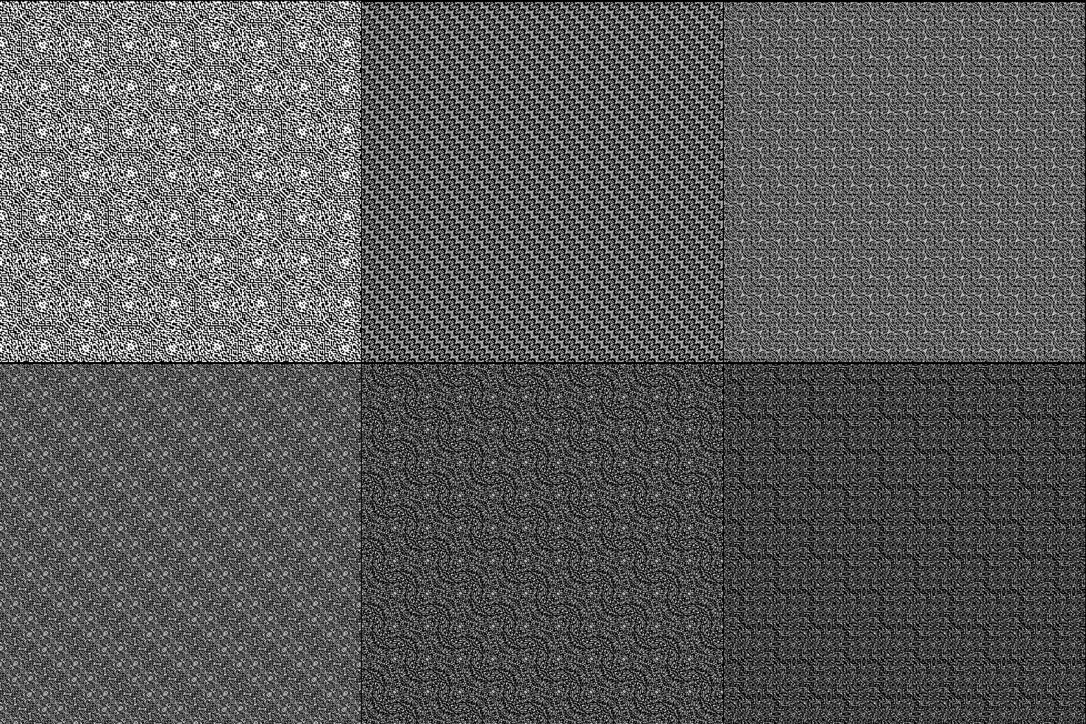
recip_various

1/n in various bases (animated gif)


Spinnietzsche

• An der Trauerfeier war im Sinn Nietzsches die sonnige Stille dieser Natureinsamkeit; das Licht spielte durch die Pflaumenbäume an die Kirchmauer und bis in die helle Gruft hinein; eine grosse Spinne spann ihre Gewebe über das Grab von Ästchen zu Ästchen in einem Sonnenstrahl. — Harry Graf Kessler

   • What was Nietzschean in the service was the sunny stillness of this natural solitude: the light playing through the plum trees on the church wall and even in the grave; a large spider spinning her web over the grave from branch to branch in a sunbeam. — Nietzsche is Dead

Get Your Prox Off #2

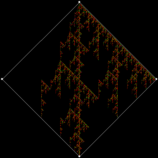
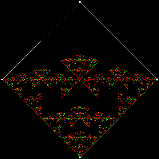
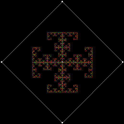
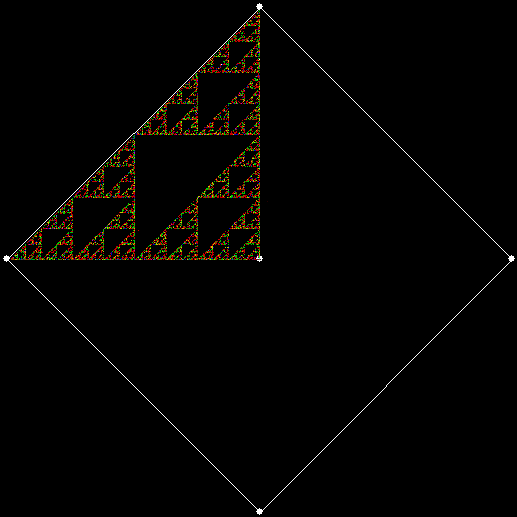
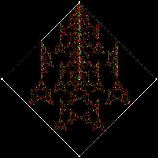
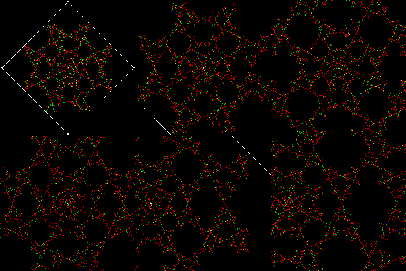
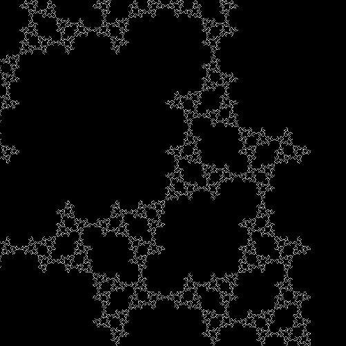
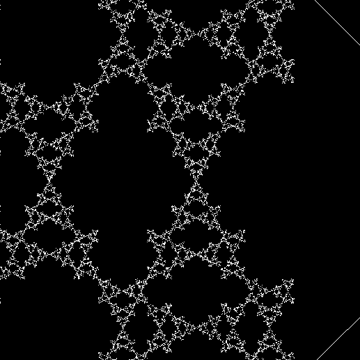
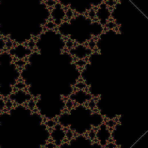
Serendipity is the art of making happy discoveries by accident. I made a mistake writing a program to create fractals and made the happy discovery of an attractive new fractal. And also of a new version of an attractive fractal I had seen before.

As I described in Get Your Prox Off, you can create a fractal by 1) moving a point towards a randomly chosen vertex of a polygon, but 2) forbidding a move towards the nearest vertex or the second-nearest vertex or third-nearest, and so on. If the polygon is a square, the four possible basic fractals look like this (note that the first fractal is also produced by banning a move towards a vertex that was chosen in the previous move):

v4_ban1

v = 4, ban = prox(1)
(ban move towards nearest vertex)


v4_ban2

v = 4, ban = prox(2)
(ban move towards second-nearest vertex)


v4_ban3

v = 4, ban = prox(3)


v4_ban4

v = 4, ban = prox(4)


This program has to calculate what might be called the order of proximity: that is, it creates an array of distances to each vertex, then sorts the array by increasing distance. I was using a bubble-sort, but made a mistake so that the program ran through the array only once and didn’t complete the sort. If this happens, the fractals look like this (note that vertex 1 is on the right, with vertex 2, 3 and 4 clockwise from it):
v4_ban1_sw1

v = 4, ban = prox(1), sweep = 1


v4_ban2_sw1

v = 4, ban = prox(2), sweep = 1


v4_ban3_sw1

v = 4, ban = prox(3), sweep = 1


v4_ban3_sw1_anim

(Animated version of v4, ban(prox(3)), sw=1)


v4_ban4_sw1

v = 4, ban = prox(4), sweep = 1


Note that in the last case, where ban = prox(4), a bubble-sort needs only one sweep to identify the most distant vertex, so the fractal looks the same as it does with a complete bubble-sort.

These new fractals looked interesting, so I had the idea of adjusting the number of sweeps in the incomplete bubble-sort: one sweep or two or three and so on (with enough sweeps, the bubble-sort becomes complete, but more sweeps are needed to complete a sort as the number of vertices increases). If there are two sweeps, then ban(prox(1)) and ban(prox(2)) look like this:

v4_ban1_sw2

v = 4, ban = prox(1), sweep = 2


v4_ban2_sw1

v = 4, ban = prox(2), sweep = 2


But the fractals produced by sweep = 2 for ban(prox(3)) and ban(prox(4)) are identical to the fractals produced by a complete bubble sort. Now, suppose you add a central point to the polygon and treat that as an additional vertex. If the bubble-sort is incomplete, a ban(prox(1)) fractal with a central point looks like this:

v4c_ban1_sw1

v = 4+c, ban = prox(1), sw = 1


v4c_ban1_sw2

v = 4+c, ban = prox(1), sw = 2


When sweep = 3, an attractive new fractal appears:

v4c_ban1_sw3

v = 4+c, ban = prox(1), sw = 3


v4c_ban1_sw3_anim

v = 4+c, ban = prox(1), sw = 3 (animated)


If you ban two vertices, the nearest and second-nearest, i.e. ban(prox(1), prox(2)), a complete bubble-sort produces a familiar fractal:

v4_ban12

v = 4+c, ban = prox(1), prox(2)


And here is ban(prox(2), prox(4)), with a complete bubble-sort:

v4c_ban24

v = 4, ban = prox(2), prox(4)


If the bubble-sort is incomplete, sweep = 1 and sweep = 2 produce these fractals for ban(prox(1), prox(2)):

v4_ban12_sw1

v = 4, ban = prox(1), prox(2), sw = 1


v4_ban12_sw2

v = 4, ban = prox(1), prox(2), sw = 2*

*The second of those fractals is identical to v = 4, ban(prox(2), prox(3)) with a complete bubble-sort.


Here is ban(prox(1), prox(5)) with a complete bubble-sort:

4c_ban15

v = 4, ban = prox(1), prox(5)


Now try ban(prox(1), prox(5)) with an incomplete bubble-sort:

v4_ban15_sw1

v = 4, ban = prox(1), prox(5), sw = 1


v4_ban15_sw2

v = 4, ban = prox(1), prox(5), sw = 2


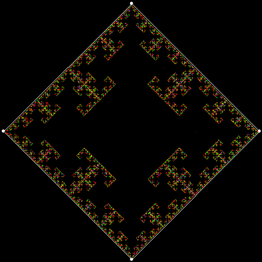
When sweep = 3, the fractal I had seen before appears:

v4_ban15_sw3

v = 4, ban = prox(1), prox(5), sw = 3


v4_ban15_sw3_anim

v = 4, ban = prox(1), prox(5), sw = 3 (animated)


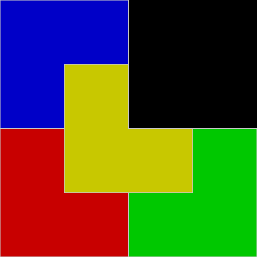
Where had I seen it before? While investigating this rep-tile (a shape that can be tiled with smaller versions of itself):

L-reptile

L-triomino rep-tile


L-reptile_anim

L-triomino rep-tile (animated)


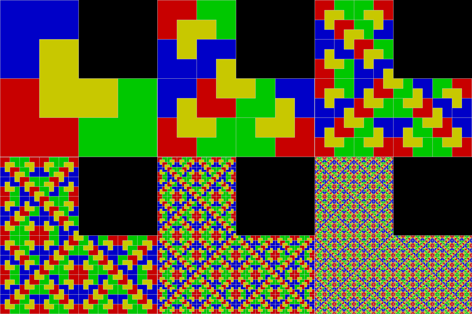
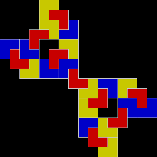
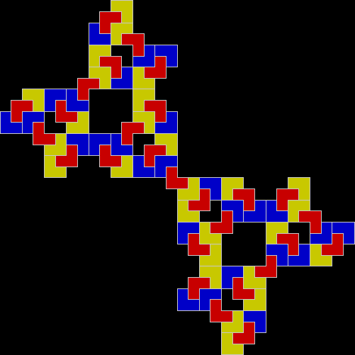
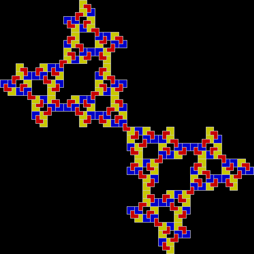
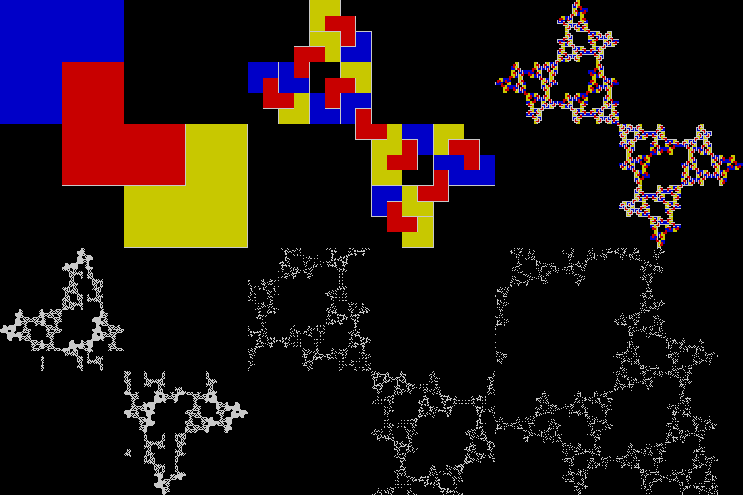
The rep-tile is technically called an L-triomino, because it looks like a capital L and is one of the two distinct shapes you can create by joining three squares at the edges. You can create fractals from an L-triomino by dividing it into four copies, discarding one of the copies, then repeating the divide-and-discard at smaller and smaller scales:

L-reptile_1

L-triomino fractal stage #1


L-reptile_2

L-triomino fractal stage #2


L-reptile_3

L-triomino fractal stage #3


L-reptile_4

L-triomino fractal stage #4


L-reptile_5

L-triomino fractal stage #5


L-reptile_fractal_anim

L-triomino fractal (animated)

L-reptile_fractal_static

L-triomino fractal (close-up)

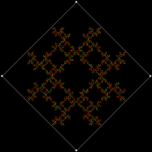
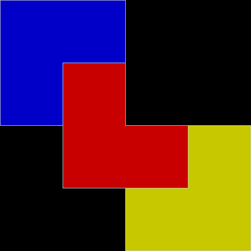
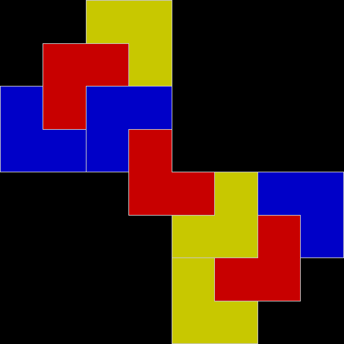
And here’s part of the ban(prox(1), prox(5)) fractal for comparison:

v4_ban15_sw3_mono


v4_ban15_sw3_col

So you can get to the same fractal (or versions of it), by two apparently different routes: random movement of a point inside a square or repeatedly dividing-and-discarding the sub-copies of an L-triomino. That’s serendipity!


Previously pre-posted:

• Get Your Prox Off

Toxic Turntable #5

Currently listening…

• Westhenge, Treow (2008)
• Unvit, Swarm ov Static (1987)
• Clangor-DBL, Oculus Omnividens (1994)
• Mallambar, Iesovo (1973)
• QVH, 484 (2011)


Previously pre-posted:

Toxic Turntable #1 • #2 • #3 • #4 •