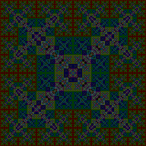
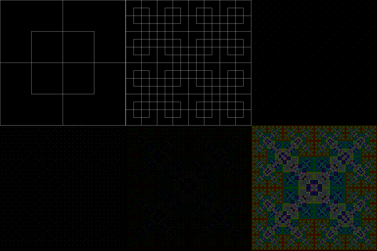
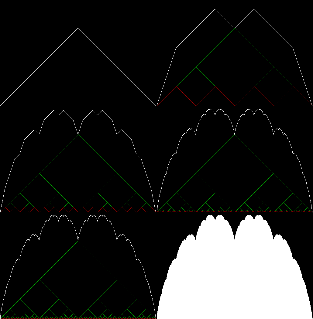
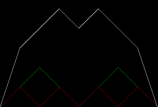
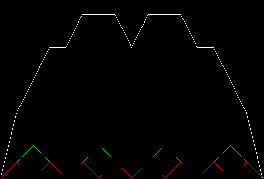
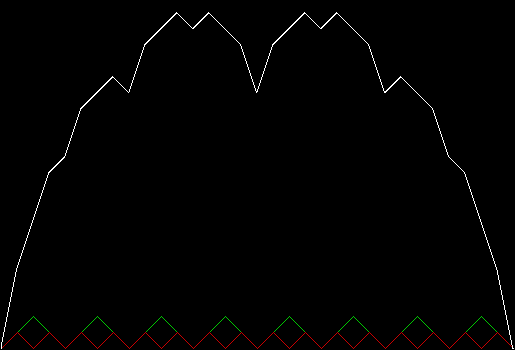
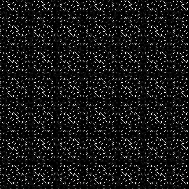
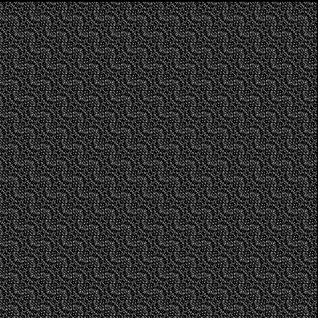
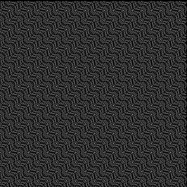
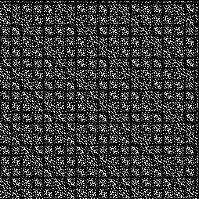
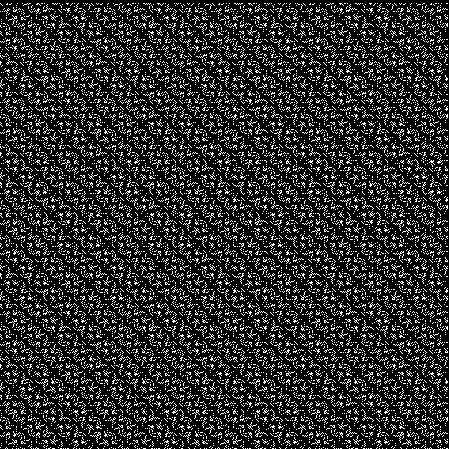
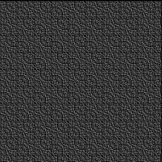
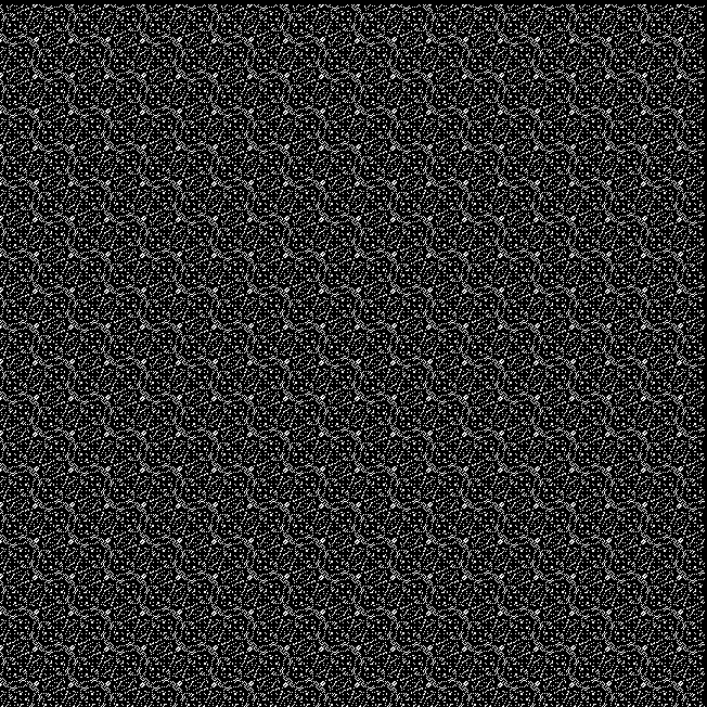
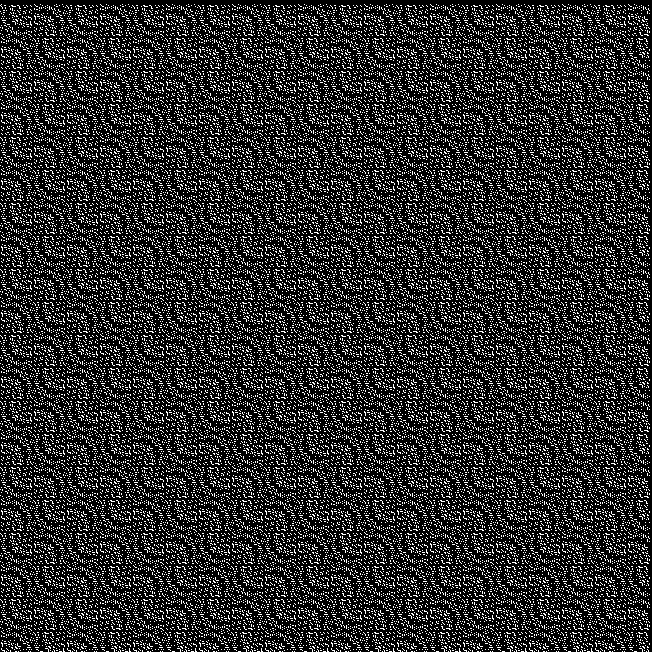
Spinnietzsche

• An der Trauerfeier war im Sinn Nietzsches die sonnige Stille dieser Natureinsamkeit; das Licht spielte durch die Pflaumenbäume an die Kirchmauer und bis in die helle Gruft hinein; eine grosse Spinne spann ihre Gewebe über das Grab von Ästchen zu Ästchen in einem Sonnenstrahl. — Harry Graf Kessler

   • What was Nietzschean in the service was the sunny stillness of this natural solitude: the light playing through the plum trees on the church wall and even in the grave; a large spider spinning her web over the grave from branch to branch in a sunbeam. — Nietzsche is Dead

Get Your Prox Off #2

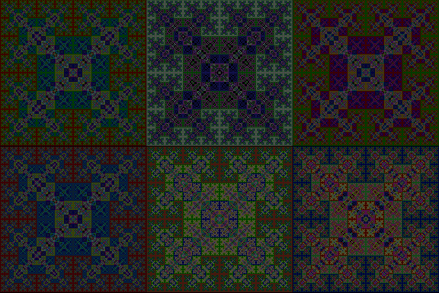
Serendipity is the art of making happy discoveries by accident. I made a mistake writing a program to create fractals and made the happy discovery of an attractive new fractal. And also of a new version of an attractive fractal I had seen before.

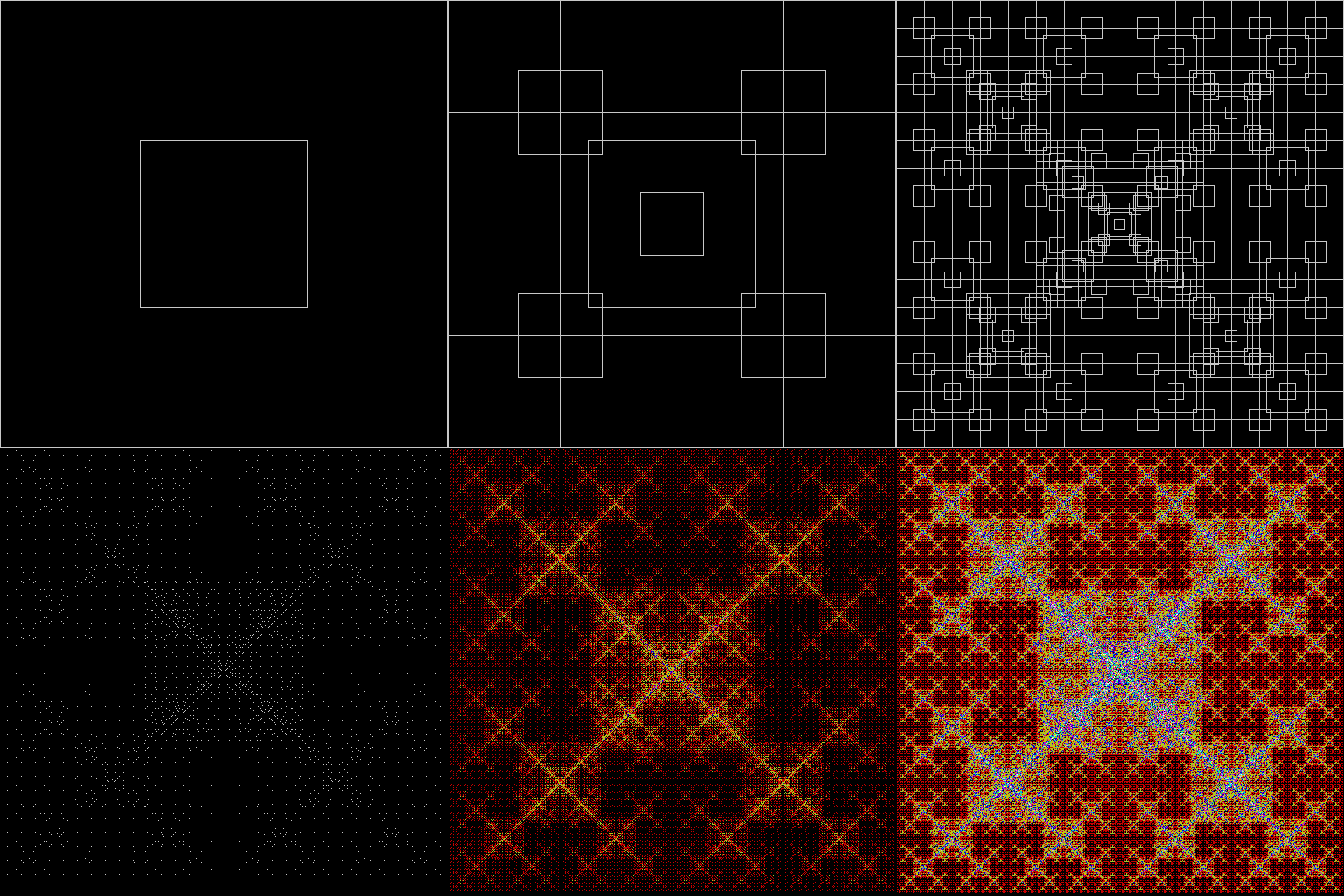
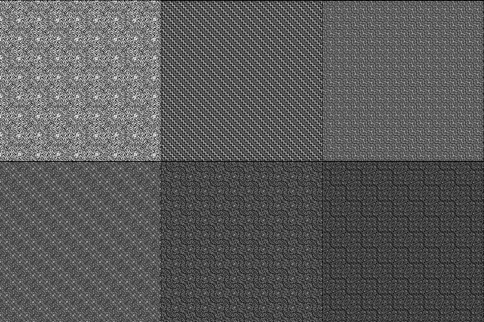
As I described in Get Your Prox Off, you can create a fractal by 1) moving a point towards a randomly chosen vertex of a polygon, but 2) forbidding a move towards the nearest vertex or the second-nearest vertex or third-nearest, and so on. If the polygon is a square, the four possible basic fractals look like this (note that the first fractal is also produced by banning a move towards a vertex that was chosen in the previous move):

v4_ban1

v = 4, ban = prox(1)
(ban move towards nearest vertex)


v4_ban2

v = 4, ban = prox(2)
(ban move towards second-nearest vertex)


v4_ban3

v = 4, ban = prox(3)


v4_ban4

v = 4, ban = prox(4)


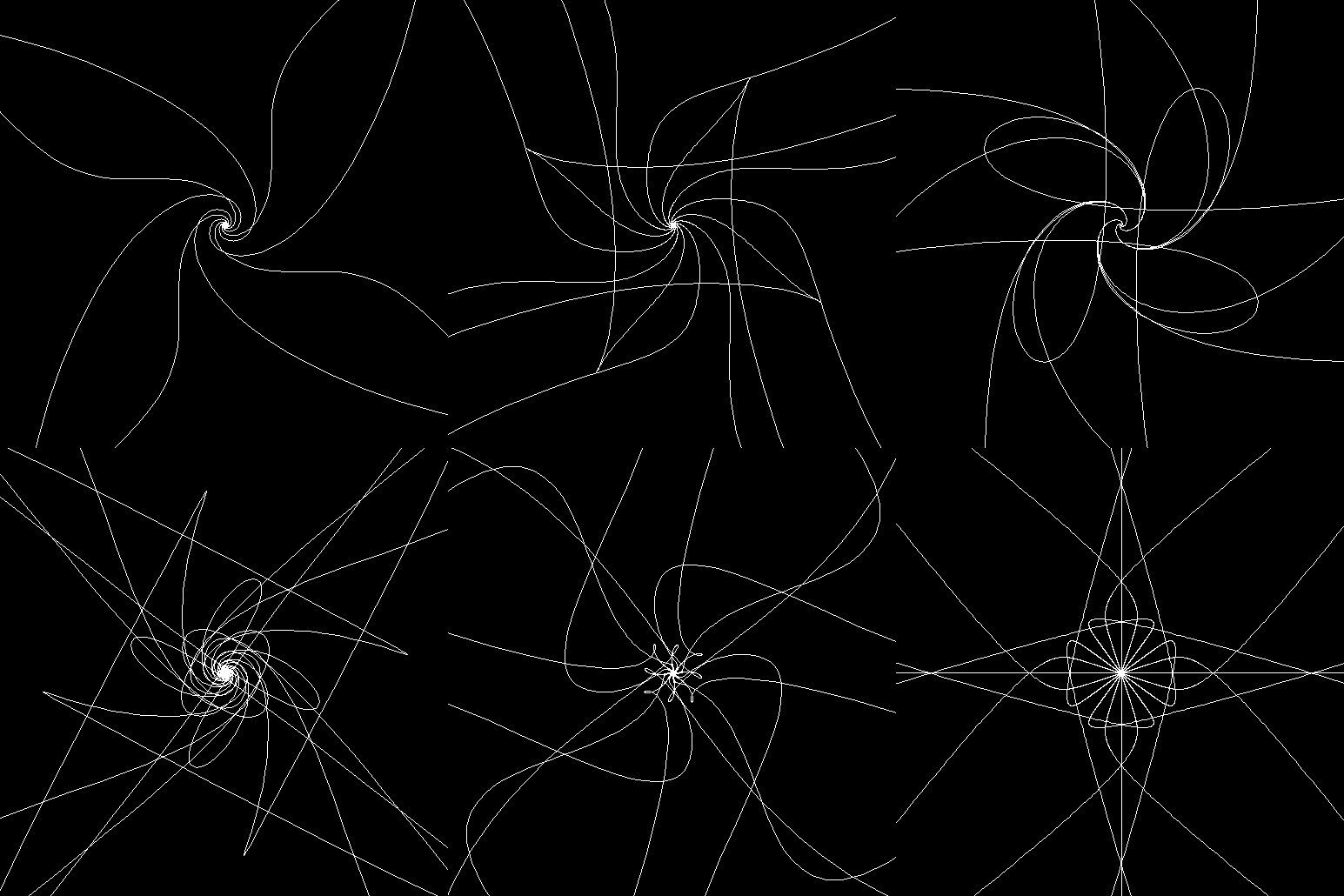
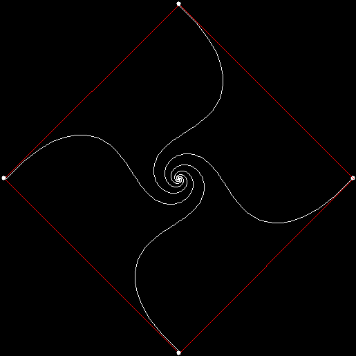
This program has to calculate what might be called the order of proximity: that is, it creates an array of distances to each vertex, then sorts the array by increasing distance. I was using a bubble-sort, but made a mistake so that the program ran through the array only once and didn’t complete the sort. If this happens, the fractals look like this (note that vertex 1 is on the right, with vertex 2, 3 and 4 clockwise from it):
v4_ban1_sw1

v = 4, ban = prox(1), sweep = 1


v4_ban2_sw1

v = 4, ban = prox(2), sweep = 1


v4_ban3_sw1

v = 4, ban = prox(3), sweep = 1


v4_ban3_sw1_anim

(Animated version of v4, ban(prox(3)), sw=1)


v4_ban4_sw1

v = 4, ban = prox(4), sweep = 1


Note that in the last case, where ban = prox(4), a bubble-sort needs only one sweep to identify the most distant vertex, so the fractal looks the same as it does with a complete bubble-sort.

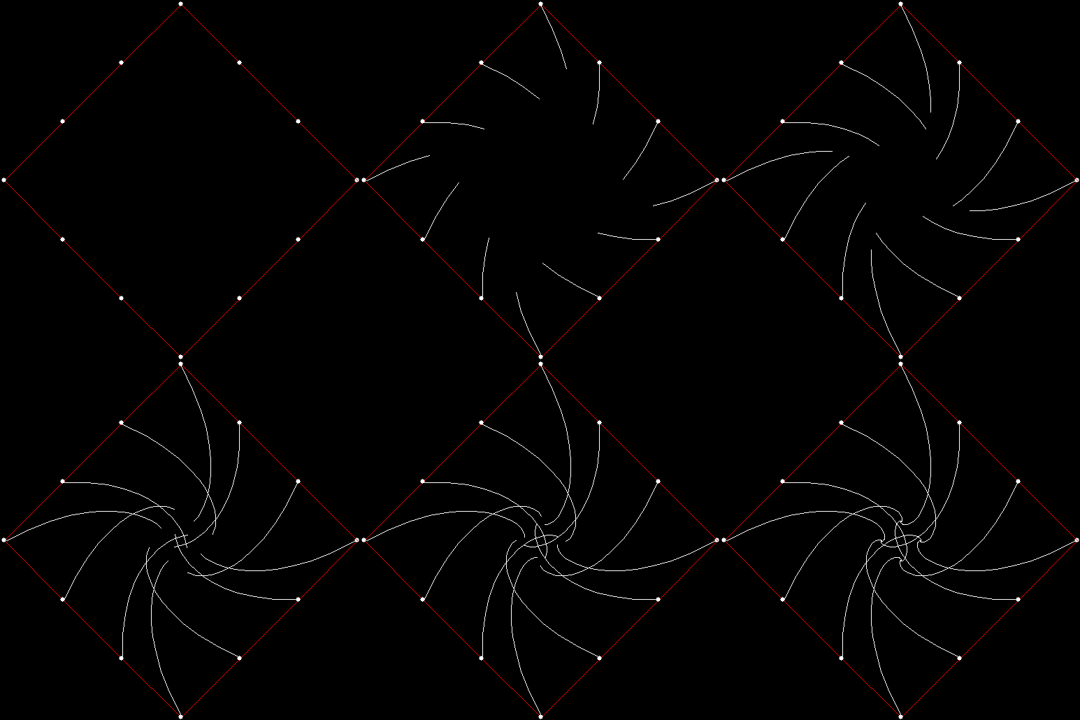
These new fractals looked interesting, so I had the idea of adjusting the number of sweeps in the incomplete bubble-sort: one sweep or two or three and so on (with enough sweeps, the bubble-sort becomes complete, but more sweeps are needed to complete a sort as the number of vertices increases). If there are two sweeps, then ban(prox(1)) and ban(prox(2)) look like this:

v4_ban1_sw2

v = 4, ban = prox(1), sweep = 2


v4_ban2_sw1

v = 4, ban = prox(2), sweep = 2


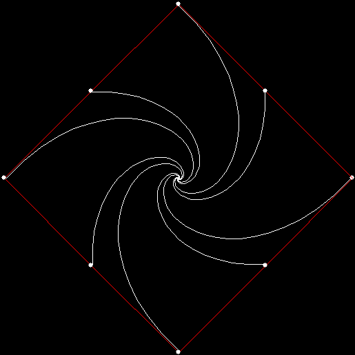
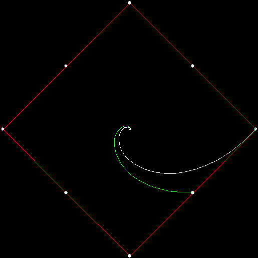
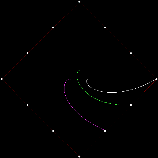
But the fractals produced by sweep = 2 for ban(prox(3)) and ban(prox(4)) are identical to the fractals produced by a complete bubble sort. Now, suppose you add a central point to the polygon and treat that as an additional vertex. If the bubble-sort is incomplete, a ban(prox(1)) fractal with a central point looks like this:

v4c_ban1_sw1

v = 4+c, ban = prox(1), sw = 1


v4c_ban1_sw2

v = 4+c, ban = prox(1), sw = 2


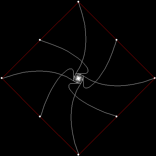
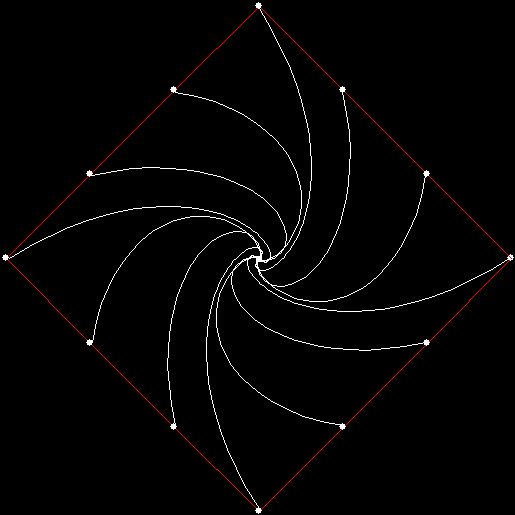
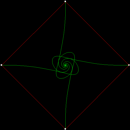
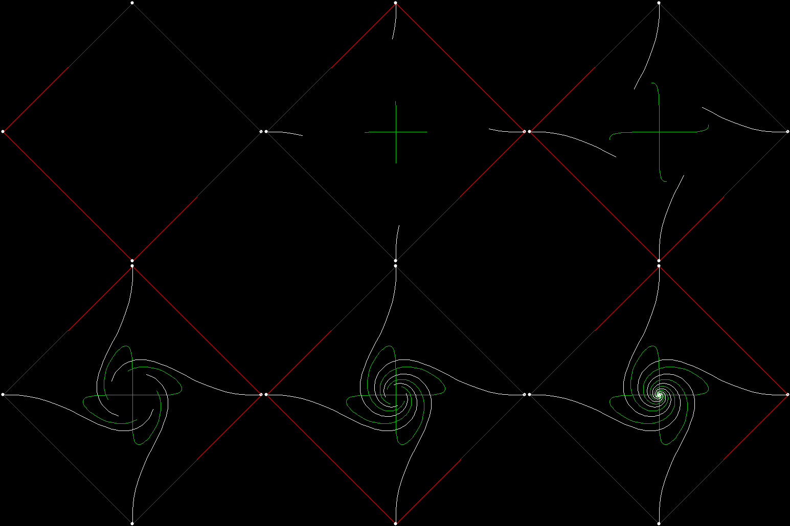
When sweep = 3, an attractive new fractal appears:

v4c_ban1_sw3

v = 4+c, ban = prox(1), sw = 3


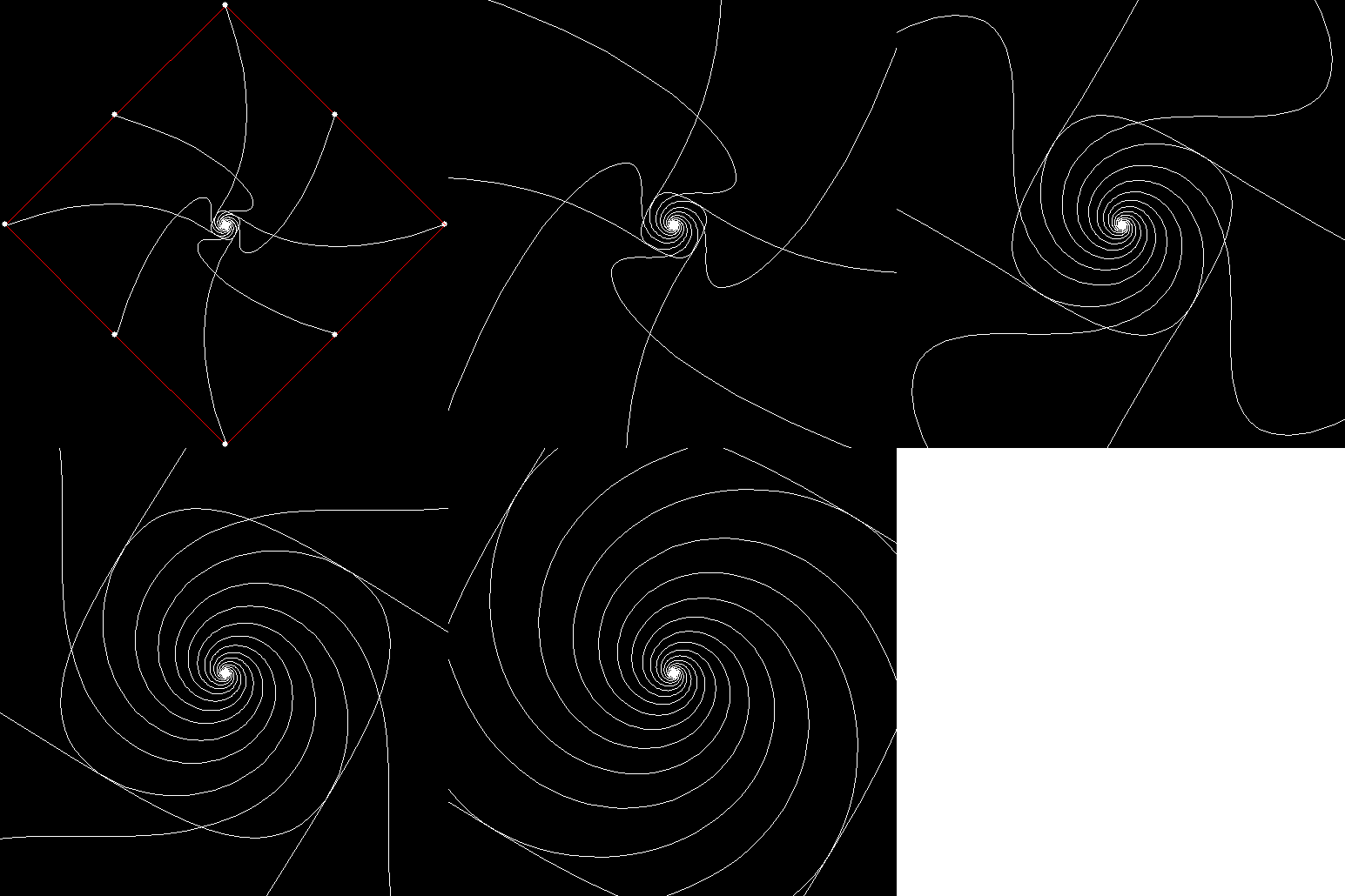
v4c_ban1_sw3_anim

v = 4+c, ban = prox(1), sw = 3 (animated)


If you ban two vertices, the nearest and second-nearest, i.e. ban(prox(1), prox(2)), a complete bubble-sort produces a familiar fractal:

v4_ban12

v = 4+c, ban = prox(1), prox(2)


And here is ban(prox(2), prox(4)), with a complete bubble-sort:

v4c_ban24

v = 4, ban = prox(2), prox(4)


If the bubble-sort is incomplete, sweep = 1 and sweep = 2 produce these fractals for ban(prox(1), prox(2)):

v4_ban12_sw1

v = 4, ban = prox(1), prox(2), sw = 1


v4_ban12_sw2

v = 4, ban = prox(1), prox(2), sw = 2*

*The second of those fractals is identical to v = 4, ban(prox(2), prox(3)) with a complete bubble-sort.


Here is ban(prox(1), prox(5)) with a complete bubble-sort:

4c_ban15

v = 4, ban = prox(1), prox(5)


Now try ban(prox(1), prox(5)) with an incomplete bubble-sort:

v4_ban15_sw1

v = 4, ban = prox(1), prox(5), sw = 1


v4_ban15_sw2

v = 4, ban = prox(1), prox(5), sw = 2


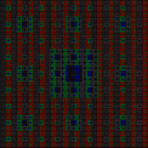
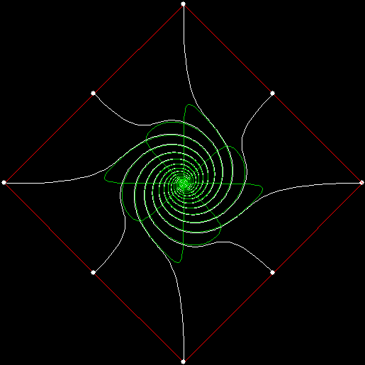
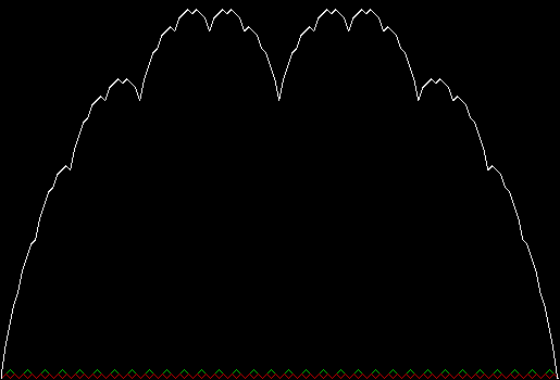
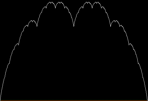
When sweep = 3, the fractal I had seen before appears:

v4_ban15_sw3

v = 4, ban = prox(1), prox(5), sw = 3


v4_ban15_sw3_anim

v = 4, ban = prox(1), prox(5), sw = 3 (animated)


Where had I seen it before? While investigating this rep-tile (a shape that can be tiled with smaller versions of itself):

L-reptile

L-triomino rep-tile


L-reptile_anim

L-triomino rep-tile (animated)


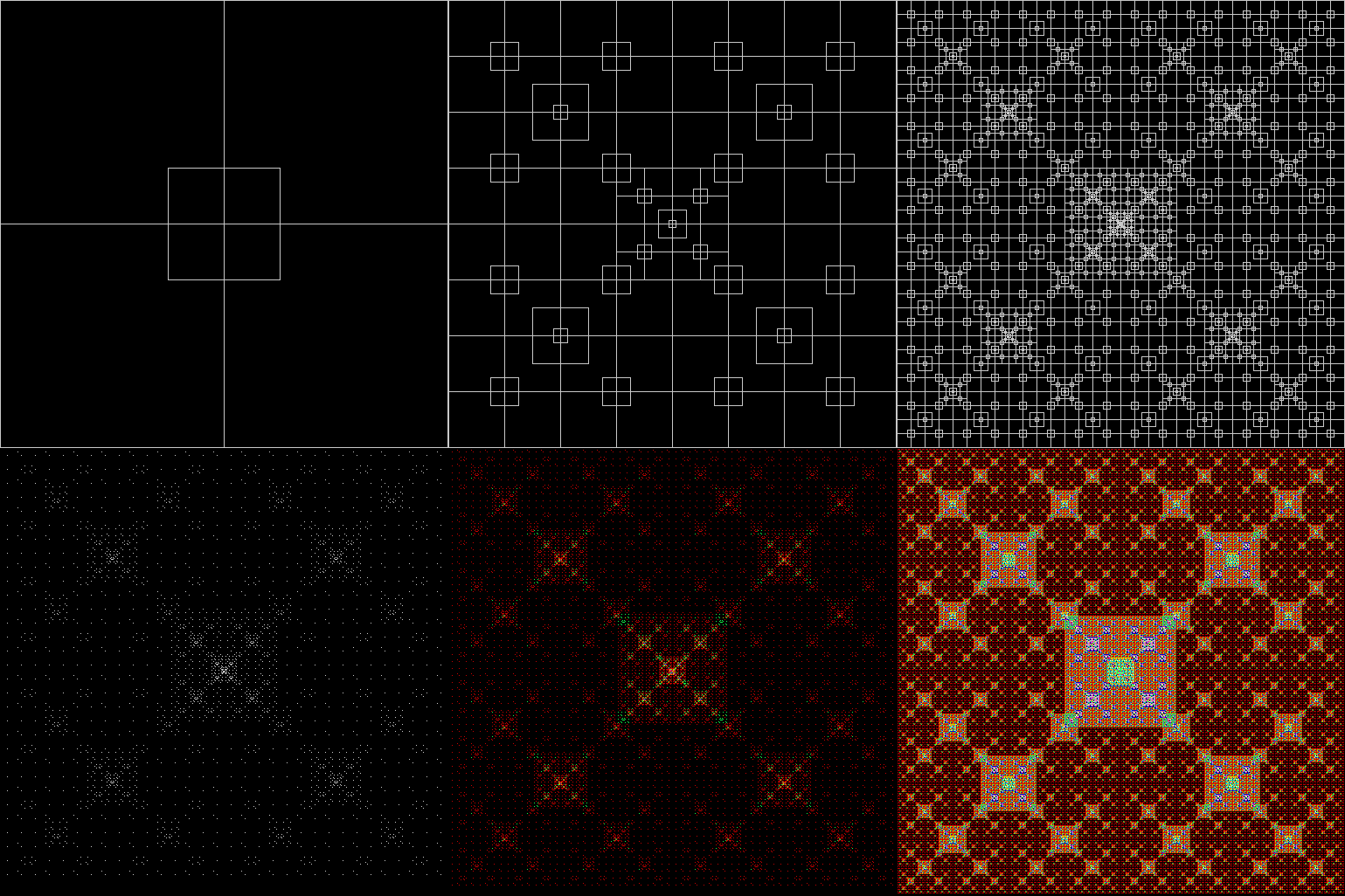
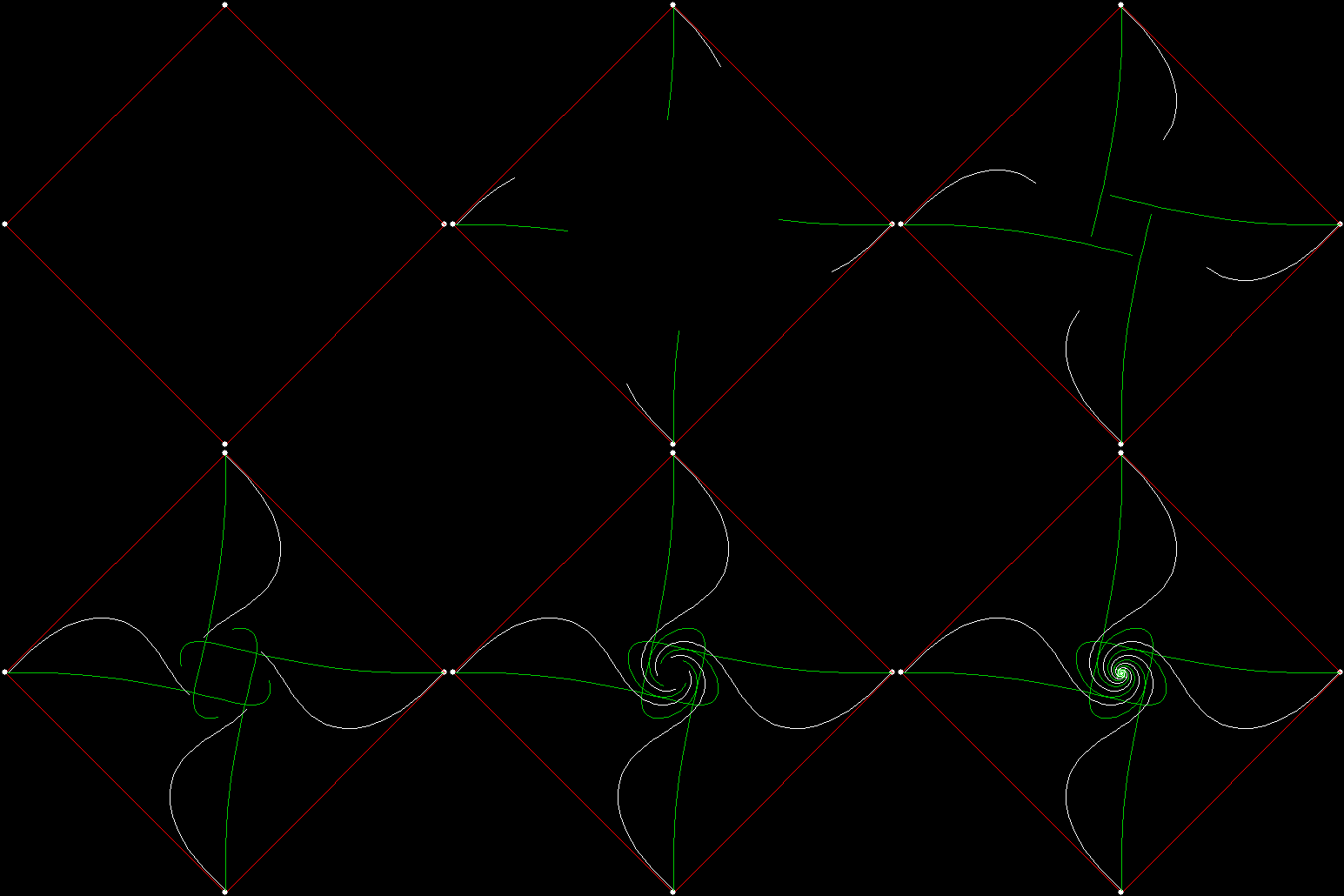
The rep-tile is technically called an L-triomino, because it looks like a capital L and is one of the two distinct shapes you can create by joining three squares at the edges. You can create fractals from an L-triomino by dividing it into four copies, discarding one of the copies, then repeating the divide-and-discard at smaller and smaller scales:

L-reptile_1

L-triomino fractal stage #1


L-reptile_2

L-triomino fractal stage #2


L-reptile_3

L-triomino fractal stage #3


L-reptile_4

L-triomino fractal stage #4


L-reptile_5

L-triomino fractal stage #5


L-reptile_fractal_anim

L-triomino fractal (animated)

L-reptile_fractal_static

L-triomino fractal (close-up)

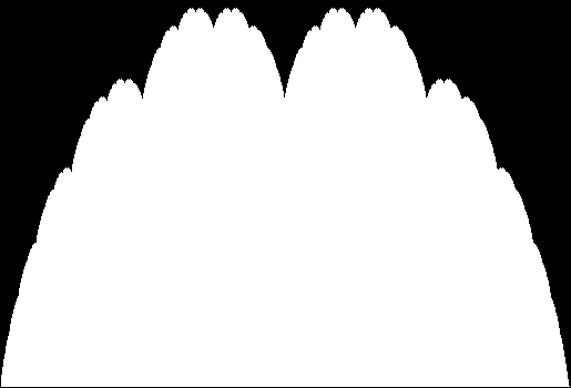
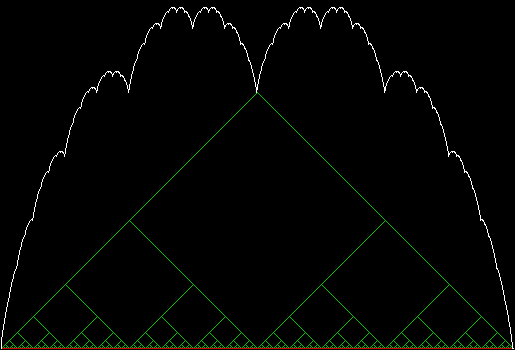
And here’s part of the ban(prox(1), prox(5)) fractal for comparison:

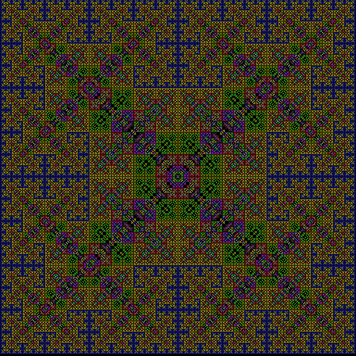
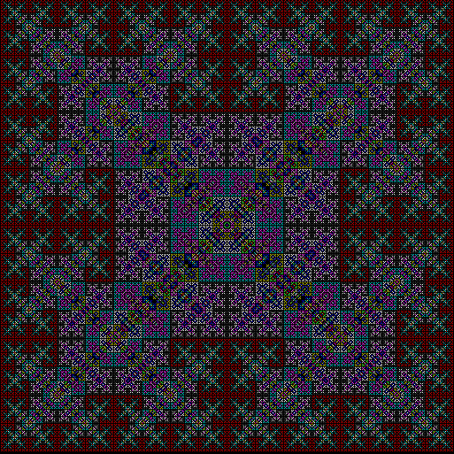
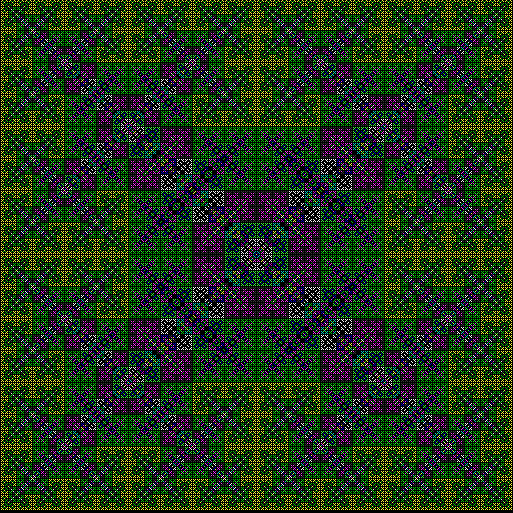
v4_ban15_sw3_mono


v4_ban15_sw3_col

So you can get to the same fractal (or versions of it), by two apparently different routes: random movement of a point inside a square or repeatedly dividing-and-discarding the sub-copies of an L-triomino. That’s serendipity!


Previously pre-posted:

Get Your Prox Off

Toxic Turntable #5

Currently listening…

• Westhenge, Treow (2008)
• Unvit, Swarm ov Static (1987)
• Clangor-DBL, Oculus Omnividens (1994)
• Mallambar, Iesovo (1973)
• QVH, 484 (2011)


Previously pre-posted:

Toxic Turntable #1#2#3#4

Performativizing Papyrocentricity #48

Papyrocentric Performativity Presents:

Vois la ReinePhilip’s Moon Observer’s Guide, Peter Grego (Philip’s 2015)

Gods of FireVolcano Discoveries: A Photographic Journey around the World, Tom Pfeiffer and Ingrid Smet (New Holland 2015)

Chemical TalesRocks and Minerals, Ronald Louis Bonewitz (Dorling Kindersley 2012)

Knyghtes of the RoyalmeMalory: Works, ed. Eugène Vinaver (Oxford University Press 1977)

Alfredo to ZinedineFootball’s Great Heroes and Entertainers, Jimmy Greaves with Norman Giller (Hodder & Stoughton 2007)


Or Read a Review at Random: RaRaR

He Say, He Sigh, He Sow #37

• Il sole, con tutti quei pianeti che girano intorno ad esso e da esso dipendono, può ancora maturare un grappolo d’uva come se non vi fosse nient’altro da fare in tutto l’universo. — Galileo Galilei, 1564-1642.

   • “The sun, with all those planets turning around it and dependent on it, can still ripen a bunch of grapes as if it had nothing else in the universe to do.”

Match of the Day

Some interesting shapes are mentioned in Derrick Niederman’s Number Freak (2010). Using identical matchsticks, what’s the smallest fully connected shape you can make in which two matches meet at every vertex? That is, what is the smallest 2-regular matchstick graph?

It’s an equilateral triangle:

2match

Now, what is the smallest fully connected shape you can make in which three matches meet at every vertex? That is, what is the smallest 3-regular matchstick graph? It uses twelve identical matches and looks like this:

3match

And here is the smallest known 4-regular matchstick graph, discovered by the German mathematician Heiko Harborth and using 104 identical matches:

4match

But Niederman says that “it’s impossible to create any arrangement in which five or more matchsticks meet at every vertex” (entry for “104”, pg. 230 of the 2012 paperback).

Radical Sheet

If you take a sheet of standard-sized paper and fold it in half from top to bottom, the folded sheet has the same proportions as the original, namely √2 : 1. In other words, if x = √2 / 2, then 1 / x = √2:

√2 = 1.414213562373…, √2 / 2 = 0.707106781186…, 1 / 0.707106781186… = 1.414213562373…

So you could say that paper has radical sheet (the square or other root of a number is also called its radix and √ is known as the radical sign). When a rectangle has the proportions √2 : 1, it can be tiled with an infinite number of copies of itself, the first copy having ½ the area of the original, the second ¼, the third ⅛, and so on. The radical sheet below is tiled with ten diminishing copies of itself, the final two having the same area:

papersizes

papersizes_static

You can also tile a radical sheet with six copies of itself, two copies having ¼ the area of the original and four having ⅛:

paper_6div_static

paper_6div

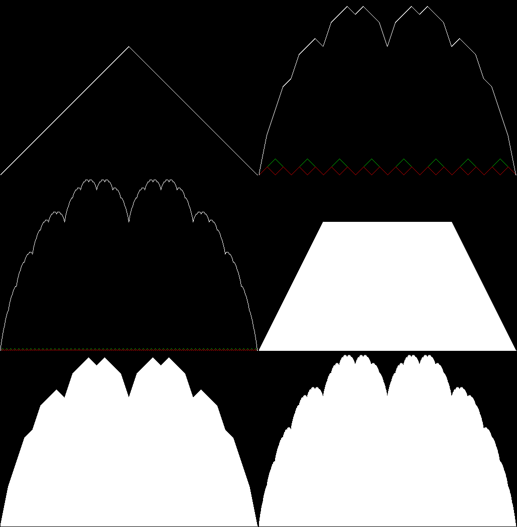
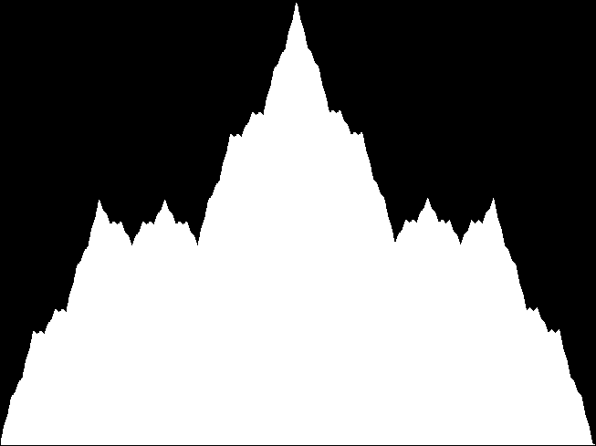
This tiling is when you might say the radical turns crucial, because you can create a fractal cross from it by repeatedly dividing and discarding. Suppose you divide a radical sheet into six copies as above, then discard two of the ⅛-sized rectangles, like this:

paper_cross_1

Stage 1


Then repeat with the smaller rectangles:

paper_cross_2

Stage 2


paper_cross_3

Stage 3


paper_cross_4

Stage 4


paper_cross_5

Stage 5


paper_cross

Animated version

paper_cross_static

Fractile cross

The cross is slanted, but it’s easy to rotate the original rectangle and produce an upright cross:

paper_cross_upright

paper_cross_upright_static

Performativizing the Polygonic

Maths is a mountain: you can start climbing in different places and reach the same destination. There are many ways of proving the irrationality of √2 or the infinitude of the primes, for example. But you can also arrive at the same destination by accident. I’ve found that when I use different methods of creating fractals. The same fractals appear, because apparently different algorithms are actually the same underneath.

But different methods can create unique fractals too. I’ve found some new ones by using what might be called point-to-point recursion. For example, there are ten ways to select three vertices from the five vertices of a pentagon: (1, 2, 3), (1, 2, 4), (1, 2, 5), (1, 3, 4), (1, 3, 5), (1, 4, 5), (2, 3, 4), (2, 3, 5), (2, 4, 5), (3, 4, 5). Find the midpoint of the first three-point set, (1, 2, 3). Then select two vertices to go with this midpoint, creating a new three-point set, and find the midpoint again. And so on. The process looks like this, with the midpoints shown for all the three-point sets found at each stage:

v5_p3_stage1

vertices = 5, choose sets of 3 points, find mid-point of each

v5_p3_stage2

v5_p3_stage3


At stage 5, the fractal looks like this:

v5_p3_static

v = 5, p = 3


Note that when pixels are used again, the colour changes. That’s another interesting thing about maths: limits can sometimes produce deeper results. If these fractals were drawn at very high resolution, pixels would only be used once and the colour would never change. As it is, low resolution means that pixels are used again and again. But some are used more than others, which is why interesting colour effects appear.

If the formation of the fractal is animated, it looks like this (with close-ups of even deeper stages):
v5_p3


Here are some more examples:

v4c_p2_static

v = 4 + central point, p = 2 (cf. Fingering the Frigit)

v4c_p2

v = 4c, p = 2 (animated)


v4_p3_static

v = 4, p = 3

v4_p3


v5_p4_static

v = 5, p = 4

v5_p4


v5c_p3_static

v = 5 + central point, p = 3

v5c_p3


v5c_p4

v = 5c, p = 4


v5c_p5

v = 5c, p = 5


v6_1_p6

v = 6 + 1 point between each pair of vertices, p = 6


v6_p2

v = 6, p = 2


v6_p3_static

v = 6, p = 3

v6_p3


v6_p4

v = 6, p = 4


v6c_p2_static

v = 6c, p = 2 (cf. Fingering the Frigit)

v6c_p2


v6c_p3_static

v = 6c, p = 3

v6c_p3


v6c_p4

v = 6c, p = 4


v7_p3

v = 7, p = 3


v7_p4_static

v = 7, p = 4

v7_p4


v7_p5_static

v = ,7 p = 5

v7_p5


v7_p4

v = 7c, p = 4


v3_1_p2

v = 3+1, p = 2


v3_1_p3

v = 3+1, p = 3


v3_1_p4

v = 3+1, p = 4


v3_2_p5

v = 3+2, p = 5


v3c_1_p2

v = 3c+1, p = 2


v3c_1_p4

v = 3c+1, p = 4


v3c_p2

v = 3c, p = 2


v3c_p3

v = 3c, p = 3


v4_1_p3

v = 4+1, p = 3


v4_1_p4

v = 4+1, p = 4


v4_1_p5

v = 4+1, p = 6


v4_1_p6

v = 4+1, p = 2


v4c_1_p4

v = 4c+1, p = 4


v4c_p3_static

v = 4c, p = 3

v4c_p3


v5_1_p4_va

v = 5+1, p = 4 (and more)


v5_p2

v = 5, p = 2


I Have a Threem

And now I have another. My first “threem”, or “three-M”, for this bijou bloguette was the alliterative three-word Latin phrase Mathematica Magistra Mundi, meaning “Mathematics Mistress of the World”. I also use it in the form Mathematica Machina Mundi, which has a variety of translations. In both Latin phrases, the words have five, three and two syllables, respectively. That’s the first three prime numbers in reverse and also part of the Fibonacci sequence in reverse.
You can find the same alliteration in languages derived from Latin, like the French La Mathématique, Maîtresse du Monde, but you don’t get the same syllable-count. So how likely was it that everything – the same alliteration and the same syllable-count – would appear in a language unrelated to Latin? But it does. Here’s a Georgian translation of the threem:

მათემატიკა მსოფლიოს მეფე

Matemat’ik’a Msoplios Mepe

“Mathematics the World’s King”

Msoplios isn’t a typo: Georgian is famous for its exotic consonant clusters and მს- / ms- isn’t a particularly unusual example. But it’s one I particularly like.